This post was written jointly with David Drukker, Director of Econometrics, StataCorp.

In our last post, we introduced the concept of treatment effects and demonstrated four of the treatment-effects estimators that were introduced in Stata 13.  Today, we will talk about two more treatment-effects estimators that use matching.

Introduction

Last time, we introduced four estimators for estimating the average treatment effect (ATE) from observational data.  Each of these estimators has a different way of solving the missing-data problem that arises because we observe only the potential outcome for the treatment level received.  Today, we introduce estimators for the ATE that solve the missing-data problem by matching.

Matching pairs the observed outcome of a person in one treatment group with the outcome of the “closest” person in the other treatment group. The outcome of the closest person is used as a prediction for the missing potential outcome. The average difference between the observed outcome and the predicted outcome estimates the ATE.

What we mean by “closest” depends on our data. Matching subjects based on a single binary variable, such as sex, is simple: males are paired with males and females are paired with females. Matching on two categorical variables, such as sex and race, isn’t much more difficult. Matching on continuous variables, such as age or weight, can be trickier because of the sparsity of the data. It is unlikely that there are two 45-year-old white males who weigh 193 pounds in a sample. It is even less likely that one of those men self-selected into the treated group and the other self-selected into the untreated group. So, in such cases, we match subjects who have approximately the same weight and approximately the same age.

This example illustrates two points. First, there is a cost to matching on continuous covariates; the inability to find good matches with more than one continuous covariate causes large-sample bias in our estimator because our matches become increasingly poor.

Second, we must specify a measure of similarity. When matching directly on the covariates, distance measures are used and the nearest neighbor selected. An alternative is to match on an estimated probability of treatment, known as the propensity score.

Before we discuss estimators for observational data, we note that matching is sometimes used in experimental data to define pairs, with the treatment subsequently randomly assigned within each pair. This use of matching is related but distinct.

Nearest-neighbor matching

Nearest-neighbor matching (NNM) uses distance between covariate patterns to define “closest”. There are many ways to define the distance between two covariate patterns. We could use squared differences as a distance measure, but this measure ignores problems with scale and covariance. Weighting the differences by the inverse of the sample covariance matrix handles these issues. Other measures are also used, but these details are less important than the costs and benefits of NNM dropping the functional-form assumptions (linear, logit, probit, etc.) used in the estimators discussed last time.

Dropping the functional-form assumptions makes the NNM estimator much more flexible; it estimates the ATE for a much wider class of models. The cost of this flexibility is that the NNM estimator requires much more data and the amount of data it needs grows with each additional continuous covariate.

In the previous blog entry, we used an example of mother’s smoking status on birthweight. Let’s reconsider that example.

. webuse cattaneo2.dta, clear

Now, we use teffects nnmatch to estimate the ATE by NNM.

. teffects nnmatch (bweight mmarried mage fage medu prenatal1) (mbsmoke)

Treatment-effects estimation                    Number of obs      =      4642
Estimator      : nearest-neighbor matching      Matches: requested =         1
Outcome model  : matching                                      min =         1
Distance metric: Mahalanobis                                   max =        16
------------------------------------------------------------------------------
             |              AI Robust
     bweight |      Coef.   Std. Err.      z    P>|z|     [95% Conf. Interval]
-------------+----------------------------------------------------------------
ATE          |
     mbsmoke |
    (smoker  |
         vs  |
 nonsmoker)  |  -210.5435   29.32969    -7.18   0.000    -268.0286   -153.0584
------------------------------------------------------------------------------

The estimated ATE is -211, meaning that infants would weigh 211 grams less when all mothers smoked than when no mothers smoked.

The output also indicates that ties in distance caused at least one observation to be matched with 16 other observations, even though we requested only matching. NNM averages the outcomes of all the tied-in-distance observations, as it should. (They are all equally good and using all of them will reduce bias.)

NNM on discrete covariates does not guarantee exact matching. For example, some married women could be matched with single women. We probably prefer exact matching on discrete covariates, which we do now.

. teffects nnmatch (bweight mmarried mage fage medu prenatal1) (mbsmoke), ///
         ematch(mmarried prenatal1) 

Treatment-effects estimation                    Number of obs      =      4642
Estimator      : nearest-neighbor matching      Matches: requested =         1
Outcome model  : matching                                      min =         1
Distance metric: Mahalanobis                                   max =        16
------------------------------------------------------------------------------
             |              AI Robust
     bweight |      Coef.   Std. Err.      z    P>|z|     [95% Conf. Interval]
-------------+----------------------------------------------------------------
ATE          |
     mbsmoke |
    (smoker  |
         vs  |
 nonsmoker)  |  -209.5726   29.32603    -7.15   0.000    -267.0506   -152.0946
------------------------------------------------------------------------------

Exact matching on mmarried and prenatal1 changed the results a little bit.

Using more than one continuous covariate introduces large-sample bias, and we have three. The option biasadj() uses a linear model to remove the large-sample bias, as suggested by Abadie and Imbens (2006, 2011).

. teffects nnmatch (bweight mmarried mage fage medu prenatal1) (mbsmoke), ///
         ematch(mmarried prenatal1)  biasadj(mage fage medu)

Treatment-effects estimation                    Number of obs      =      4642
Estimator      : nearest-neighbor matching      Matches: requested =         1
Outcome model  : matching                                      min =         1
Distance metric: Mahalanobis                                   max =        16
------------------------------------------------------------------------------
             |              AI Robust
     bweight |      Coef.   Std. Err.      z    P>|z|     [95% Conf. Interval]
-------------+----------------------------------------------------------------
ATE          |
     mbsmoke |
    (smoker  |
         vs  |
 nonsmoker)  |  -210.0558   29.32803    -7.16   0.000    -267.5377   -152.5739
------------------------------------------------------------------------------

In this case, the results changed by a small amount. In general, they can change a lot, and the amount increases with the number of continuous
covariates.

Propensity-score matching

NNM uses bias adjustment to remove the bias caused by matching on more than one continuous covariate. The generality of this approach makes it very appealing, but it can be difficult to think about issues of fit and model specification. Propensity-score matching (PSM) matches on an estimated probability of treatment known as the propensity score. There is no need for bias adjustment because we match on only one continuous covariate. PSM has the added benefit that we can use all the standard methods for checking the fit of binary regression models prior to matching.

We estimate the ATE by PSM using teffects psmatch.

. teffects psmatch (bweight) (mbsmoke mmarried mage fage medu prenatal1 ) 

Treatment-effects estimation                    Number of obs      =      4642
Estimator      : propensity-score matching      Matches: requested =         1
Outcome model  : matching                                      min =         1
Treatment model: logit                                         max =        16
------------------------------------------------------------------------------
             |              AI Robust
     bweight |      Coef.   Std. Err.      z    P>|z|     [95% Conf. Interval]
-------------+----------------------------------------------------------------
ATE          |
     mbsmoke |
    (smoker  |
         vs  |
 nonsmoker)  |  -229.4492   25.88746    -8.86   0.000    -280.1877   -178.7107
------------------------------------------------------------------------------

The estimated ATE is now -229, larger in magnitude than the NNM estimates but not significantly so.

How to choose among the six estimatorsg

We now have six estimators:

1. RA: Regression adjustment
2. IPW: Inverse probability weighting
3. IPWRA: Inverse probability weighting with regression adjustment
4. AIPW: Augmented inverse probability weighting
5. NNM: Nearest-neighbor matching
6. PSM: Propensity-score matching

The ATEs we estimated are

1. RA: -277.06
2. IPW: -275.56
3. IPWRA: -229.97
4. AIPW: -230.99
5. NNM: -210.06
6. PSM: -229.45

Which estimator should we use?

We would never suggest searching the above table for the result that most closely fits your wishes and biases. The choice of estimator needs to be made beforehand.

So, how do we choose?

Here are some rules of thumb:

1. Under correct specification, all the estimators should produce similar results. (Similar estimates do not guarantee correct specification because all the specifications could be wrong.)
2. When you know the determinants of treatment status, IPW is a natural base-case estimator.
3. When you instead know the determinants of the outcome, RA is a natural base-case estimator.
4. The doubly robust estimators, AIPW and IPWRA, give us an extra shot at correct specification.
5. When you have lots of continuous covariates, NNM will crucially hinge on the bias adjustment, and the computation gets to be extremely difficult.
6. When you know the determinants of treatment status, PSM is another base-case estimator.
7. The IPW estimators are not reliable when the estimated treatment probabilities get too close to 0 or 1.

Final thoughts

Before we go, we reiterate the cautionary note from our last entry. Nothing about the mathematics of treatment-effects estimators magically extracts causal relationships from observational data. We cannot thoughtlessly analyze our data using Stata’s teffects commands and infer a causal relationship. The models must be supported by scientific theory.

If you would like to learn more about treatment effects in Stata, there is an entire manual devoted to the treatment-effects features in Stata 14; it includes a basic introduction, an advanced introduction, and many worked examples. In Stata, type help teffects:

.  help teffects 

Title

     [TE] teffects—Treatment-effects estimation for observational data

Syntax

… <output omitted> …

The title [TE] teffects will be in blue, which means it’s clickable. Click on it to go to the Treatment-Effects Reference Manual.

Or download the manual from our website; visit

http://www.stata.com/manuals14/te/

References

Abadie, A., and Imbens, G. W. 2006. Large sample properties of matching estimators for average treatment effects. Econometrica 74: 235–267.

Abadie, A., and Imbens, G. W. 2011. Bias-corrected matching estimators for average treatment effects. Journal of Business and Economic Statistics 29: 1–11.

Cattaneo, M. D. 2010. Efficient semiparametric estimation of multi-valued treatment effects under ignorability. Journal of Econometrics 155: 138–154.

Overview

In this post, I show how to use mlexp to estimate the degree of freedom parameter of a chi-squared distribution by maximum likelihood (ML). One example is unconditional, and another example models the parameter as a function of covariates. I also show how to generate data from chi-squared distributions and I illustrate how to use simulation methods to understand an estimation technique.

The data

I want to show how to draw data from a \(\chi^2\) distribution, and I want to illustrate that the ML estimator produces estimates close to the truth, so I use simulated data.

In the output below, I draw a \(2,000\) observation random sample of data from a \(\chi^2\) distribution with \(2\) degrees of freedom, denoted by \(\chi^2(2)\), and I summarize the results.

Example 1: Generating \(\chi^2(2)\) data

. drop _all

. set obs 2000
number of observations (_N) was 0, now 2,000

. set seed 12345

. generate y = rchi2(2)

. summarize y

    Variable |        Obs        Mean    Std. Dev.       Min        Max
-------------+---------------------------------------------------------
           y |      2,000    2.030865    1.990052   .0028283   13.88213

The mean and variance of the \(\chi^2(2)\) distribution are \(2\) and \(4\), respectively. The sample mean of \(2.03\) and the sample variance of \(3.96=1.99^2\) are close to the true values. I set the random-number seed to \(12345\) so that you can replicate my example; type help seed for details.

mlexp and the log-likelihood function

The log-likelihood function for the ML estimator for the degree of freedom parameter \(d\) of a \(\chi^2(d)\) distribution is

\[
{\mathcal L}(d) = \sum_{i=1}^N \ln[f(y_i,d)]
\]

where \(f(y_i,d)\) is the density function for the \(\chi^2(d)\) distribution. See Trivedi, 2005 and Wooldridge, 2010 for instructions to ML.

The mlexp command estimates parameters by maximizing the specified log-likelihood function. You specify the contribution of an observation to the log-likelihood function inside parentheses, and you enclose parameters inside the curly braces \(\{\) and \(\}\). I use mlexp to estimate \(d\) in example 2.

Example 2: Using mlexp to estimate \(d\)

. mlexp ( ln(chi2den({d},y)) )

initial:       log likelihood =     -  (could not be evaluated)
feasible:      log likelihood = -5168.1594
rescale:       log likelihood = -3417.1592
Iteration 0:   log likelihood = -3417.1592  
Iteration 1:   log likelihood = -3416.7063  
Iteration 2:   log likelihood = -3416.7063  

Maximum likelihood estimation

Log likelihood = -3416.7063                     Number of obs     =      2,000

------------------------------------------------------------------------------
             |      Coef.   Std. Err.      z    P>|z|     [95% Conf. Interval]
-------------+----------------------------------------------------------------
          /d |   2.033457   .0352936    57.62   0.000     1.964283    2.102631
------------------------------------------------------------------------------

The estimate of \(d\) is very close to the true value of \(2.0\), as expected.

Modeling the degree of freedom as a function of a covariate

When using ML in applied research, we almost always want to model the parameters of a distribution as a function of covariates. Below, I draw a covariate \(x\) from Uniform(0,3) distribution, specify that \(d=1+x\), and draw \(y\) from a \(\chi^2(d)\) distribution conditional on \(x\). Having drawn data from the DGP, I estimate the parameters using mlexp.

Example 3: Using mlexp to estimate \(d=a+b x_i\)

. drop _all

. set obs 2000
number of observations (_N) was 0, now 2,000

. set seed 12345

. generate x = runiform(0,3)

. generate d = 1 + x

. generate y = rchi2(d)

. mlexp ( ln(chi2den({b}*x +{a},y)) )

initial:       log likelihood =     -  (could not be evaluated)
feasible:      log likelihood = -4260.0685
rescale:       log likelihood = -3597.6271
rescale eq:    log likelihood = -3597.6271
Iteration 0:   log likelihood = -3597.6271  
Iteration 1:   log likelihood = -3596.5383  
Iteration 2:   log likelihood =  -3596.538  

Maximum likelihood estimation

Log likelihood =  -3596.538                     Number of obs     =      2,000

------------------------------------------------------------------------------
             |      Coef.   Std. Err.      z    P>|z|     [95% Conf. Interval]
-------------+----------------------------------------------------------------
          /b |   1.061621   .0430846    24.64   0.000     .9771766    1.146065
          /a |   .9524136   .0545551    17.46   0.000     .8454876     1.05934
------------------------------------------------------------------------------

The estimates of \(1.06\) and \(0.95\) are close to their true values.

mlexp makes this process easier by forming a linear combination of variables that you specify.

Example 4: A linear combination in mlexp

. mlexp ( ln(chi2den({xb: x _cons},y)) )

initial:       log likelihood =     -  (could not be evaluated)
feasible:      log likelihood = -5916.7648
rescale:       log likelihood = -3916.6106
Iteration 0:   log likelihood = -3916.6106  
Iteration 1:   log likelihood = -3621.2905  
Iteration 2:   log likelihood = -3596.5845  
Iteration 3:   log likelihood =  -3596.538  
Iteration 4:   log likelihood =  -3596.538  

Maximum likelihood estimation

Log likelihood =  -3596.538                     Number of obs     =      2,000

------------------------------------------------------------------------------
             |      Coef.   Std. Err.      z    P>|z|     [95% Conf. Interval]
-------------+----------------------------------------------------------------
           x |   1.061621   .0430846    24.64   0.000     .9771766    1.146065
       _cons |   .9524138   .0545551    17.46   0.000     .8454878     1.05934
------------------------------------------------------------------------------

The estimates are the same as in example 3, but the command was easier to write and the output is easier to read.

Done and undone

I have shown how to generate data from a \(\chi^2(d)\) distribution when \(d\) is a fixed number or a linear function of a covariate and how to estimate \(d\) or the parameters of the model for \(d\) by using mlexp.

The examples discussed above show how to use mlexp and illustrate an example of conditional maximum likelihood estimation.

mlexp can do much more than I have discussed here; see [R] mlexp for more details. Estimating the parameters of a conditional distribution is only the beginning of any research project. I will discuss interpreting these parameters in a future post.

References

Cameron, A. C., and P. K. Trivedi. 2005. Microeconometrics: Methods and applications. Cambridge: Cambridge University Press.

Wooldridge, J. M. 2010. Econometric Analysis of Cross Section and Panel Data. 2nd ed. Cambridge, Massachusetts: MIT Press.

Overview

In this post, I show how to use Monte Carlo simulations to compare the efficiency of different estimators. I also illustrate what we mean by efficiency when discussing statistical estimators.

I wrote this post to continue a dialog with my friend who doubted the usefulness of the sample average as an estimator for the mean when the data-generating process (DGP) is a \(\chi^2\) distribution with \(1\) degree of freedom, denoted by a \(\chi^2(1)\) distribution. The sample average is a fine estimator, even though it is not the most efficient estimator for the mean. (Some researchers prefer to estimate the median instead of the mean for DGPs that generate outliers. I will address the trade-offs between these parameters in a future post. For now, I want to stick to estimating the mean.)

In this post, I also want to illustrate that Monte Carlo simulations can help explain abstract statistical concepts. I show how to use a Monte Carlo simulation to illustrate the meaning of an abstract statistical concept. (If you are new to Monte Carlo simulations in Stata, you might want to see Monte Carlo simulations using Stata.)

Consistent estimator A is said to be more asymptotically efficient than consistent estimator B if A has a smaller asymptotic variance than B; see Wooldridge (2010, sec. 14.4.2) for an especially useful discussion. Theoretical comparisons can sometimes ascertain that A is more efficient than B, but the magnitude of the difference is rarely identified. Comparisons of Monte Carlo simulation estimates of the variances of estimators A and B give both sign and magnitude for specific DGPs and sample sizes.

The sample average versus maximum likelihood

Many books discuss the conditions under which the maximum likelihood (ML) estimator is the efficient estimator relative to other estimators; see Wooldridge (2010, sec. 14.4.2) for an accessible introduction to the modern approach. Here I compare the ML estimator with the sample average for the mean when the DGP is a \(\chi^2(1)\) distribution.

Example 1 below contains the commands I used. For an introduction to Monte Carlo simulations see Monte Carlo simulations using Stata, and for an introduction to using mlexp to estimate the parameter of a \(\chi^2\) distribution see Maximum likelihood estimation by mlexp: A chi-squared example. In short, the commands do the following \(5,000\) times:

1. Draw a sample of 500 observations from a \(\chi^2(1)\) distribution.
2. Estimate the mean of each sample by the sample average, and store this estimate in m_a in the dataset efcomp.dta.
3. Estimate the mean of each sample by ML, and store this estimate in m_ml in the dataset efcomp.dta.

Example 1: The distributions of the sample average and the ML estimators

. clear all
. set seed 12345
. postfile sim  mu_a mu_ml using efcomp, replace
. forvalues i = 1/5000 {
  2.     quietly drop _all
  3.     quietly set obs 500
  4.     quietly generate double y = rchi2(1)
  5.     quietly mean y 
  6.     local mu_a         =  _b[y]
  7.     quietly mlexp (ln(chi2den({d=1},y)))
  8.     local mu_ml   =  _b[d:_cons]
  9.     post sim (`mu_a') (`mu_ml') 
 10. }
. postclose sim
. use efcomp, clear 
. summarize

    Variable |        Obs        Mean    Std. Dev.       Min        Max
-------------+---------------------------------------------------------
        mu_a |      5,000    .9989277    .0620524   .7792076   1.232033
       mu_ml |      5,000    1.000988    .0401992   .8660786   1.161492

The mean of the \(5,000\) sample average estimates and the mean of the \(5,000\) ML estimates are each close to the true value of \(1.0\). The standard deviation of the \(5,000\) sample average estimates is \(0.062\), and it approximates the standard deviation of the sampling distribution of the sample average for this DGP and sample size. Similarly, the standard deviation of the \(5,000\) ML estimates is \(0.040\), and it approximates the standard deviation of the sampling distribution of the ML estimator for this DGP and sample size.

We conclude that the ML estimator has a lower variance than the sample average for this DGP and this sample size, because \(0.040\) is smaller than \(0.062\).

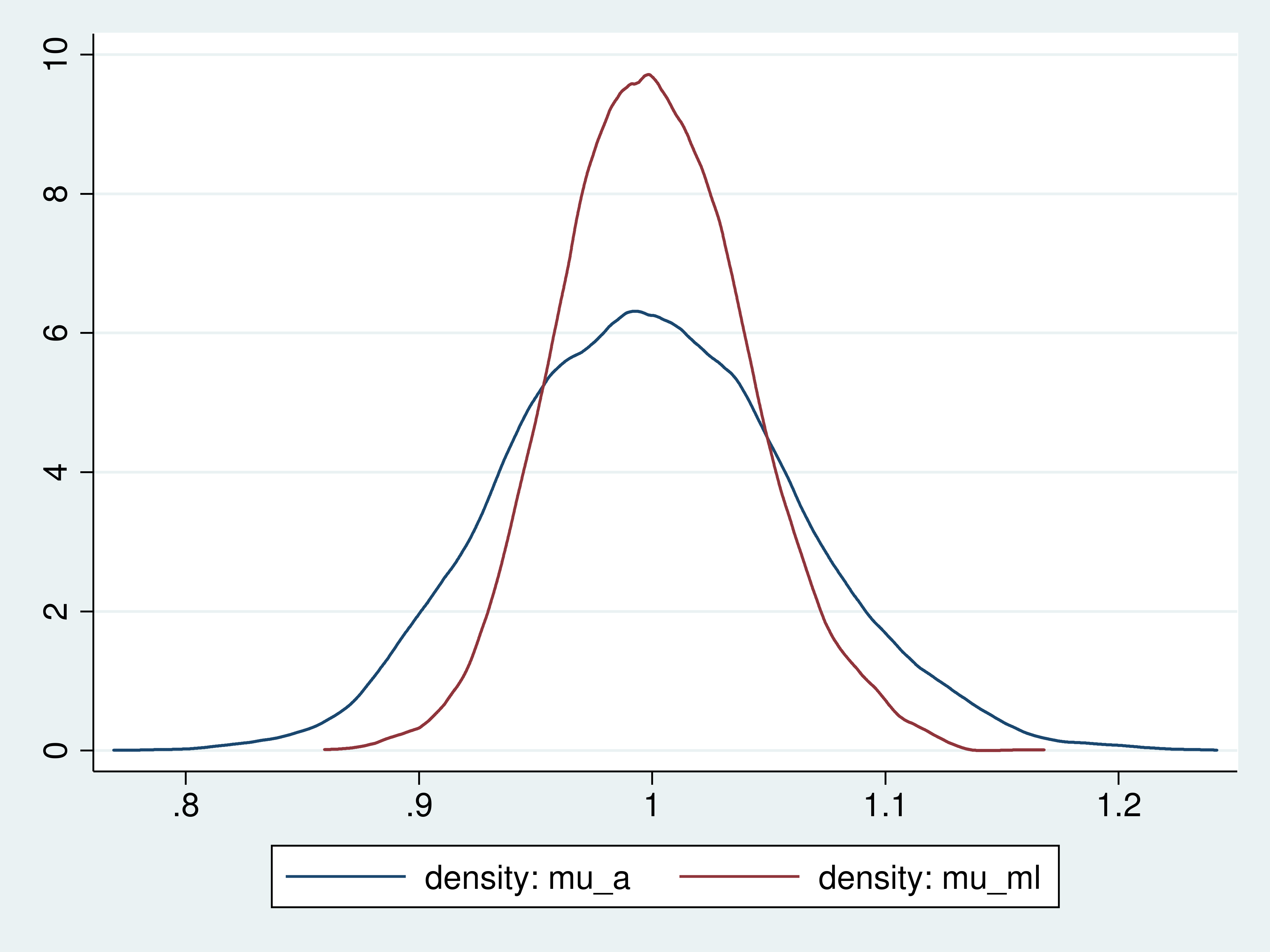
To get a picture of this difference, we plot the density of the sample average and the density of the ML estimator. (Each of these densities is estimated from \(5,000\) observations, but estimation error can be ignored because more data would not change the key results.)

Example 2: Plotting the densities of the estimators

. kdensity mu_a,   n(5000) generate(x_a   den_a)   nograph

. kdensity mu_ml,  n(5000) generate(x_ml  den_ml)  nograph

. twoway (line den_a x_a) (line den_ml x_ml)

Densities of the sample average and ML estimators

The plots show that the ML estimator is more tightly distributed around the true value than the sample average.

That the ML estimator is more tightly distributed around the true value than the sample average is what it means for one consistent estimator to be more efficient than another.

Done and undone

I used Monte Carlo simulation to illustrate what it means for one estimator to be more efficient than another. In particular, we saw that the ML estimator is more efficient than the sample average for the mean of a \(\chi^2(1)\) distribution.

Many other estimators fall between these two estimators in an efficiency ranking. Generalized method of moments estimators and some quasi-maximum likelihood estimators come to mind and might be worth adding to these simulations.

Reference

Wooldridge, J. M. 2010. Econometric Analysis of Cross Section and Panel Data. 2nd ed. Cambridge, Massachusetts: MIT Press.

\(\newcommand{\epsilonb}{\boldsymbol{\epsilon}}
\newcommand{\ebi}{\boldsymbol{\epsilon}_i}
\newcommand{\Sigmab}{\boldsymbol{\Sigma}}
\newcommand{\Omegab}{\boldsymbol{\Omega}}
\newcommand{\Lambdab}{\boldsymbol{\Lambda}}
\newcommand{\betab}{\boldsymbol{\beta}}
\newcommand{\gammab}{\boldsymbol{\gamma}}
\newcommand{\Gammab}{\boldsymbol{\Gamma}}
\newcommand{\deltab}{\boldsymbol{\delta}}
\newcommand{\xib}{\boldsymbol{\xi}}
\newcommand{\iotab}{\boldsymbol{\iota}}
\newcommand{\xb}{{\bf x}}
\newcommand{\xbit}{{\bf x}_{it}}
\newcommand{\xbi}{{\bf x}_{i}}
\newcommand{\zb}{{\bf z}}
\newcommand{\zbi}{{\bf z}_i}
\newcommand{\wb}{{\bf w}}
\newcommand{\yb}{{\bf y}}
\newcommand{\ub}{{\bf u}}
\newcommand{\Gb}{{\bf G}}
\newcommand{\Hb}{{\bf H}}
\newcommand{\thetab}{\boldsymbol{\theta}}
\newcommand{\XBI}{{\bf x}_{i1},\ldots,{\bf x}_{iT}}
\newcommand{\Sb}{{\bf S}} \newcommand{\Xb}{{\bf X}}
\newcommand{\Xtb}{\tilde{\bf X}}
\newcommand{\Wb}{{\bf W}}
\newcommand{\Ab}{{\bf A}}
\newcommand{\Bb}{{\bf B}}
\newcommand{\Zb}{{\bf Z}}
\newcommand{\Eb}{{\bf E}}\) This post was written jointly with Joerg Luedicke, Senior Social Scientist and Statistician, StataCorp.

Overview

We provide an introduction to parameter estimation by maximum likelihood and method of moments using mlexp and gmm, respectively (see [R] mlexp and [R] gmm). We include some background about these estimation techniques; see Pawitan (2001, Casella and Berger (2002), Cameron and Trivedi (2005), and Wooldridge (2010) for more details.

Maximum likelihood (ML) estimation finds the parameter values that make the observed data most probable. The parameters maximize the log of the likelihood function that specifies the probability of observing a particular set of data given a model.

Method of moments (MM) estimators specify population moment conditions and find the parameters that solve the equivalent sample moment conditions. MM estimators usually place fewer restrictions on the model than ML estimators, which implies that MM estimators are less efficient but more robust than ML estimators.

Using mlexp to estimate probit model parameters

A probit model for the binary dependent variable \(y\) conditional on covariates \(\xb\) with coefficients \(\betab\) is

\[\begin{equation}
y = \begin{cases}
1 & \mbox{ if } \xb\betab’ + \epsilon > 0\\
0 & \mbox{ otherwise }
\end{cases}
\end{equation}\]

where \(\epsilon\) has a standard normal distribution. The log-likelihood function for the probit model is

\[\begin{equation}\label{E:b1}
\ln\{L(\betab;\xb,y)\}= \sum_{i=1}^N y_i \ln\Phi(\xb_{i}\betab’)
+ (1-y_i) \ln\Phi(-\xb_{i}\betab’)
\end{equation}\]

where \(\Phi\) denotes the cumulative standard normal.

We now use mlexp to estimate the coefficients of a probit model. We have data on whether an individual belongs to a union (union), the individual’s age (age), and the highest grade completed (grade).

. webuse union
(NLS Women 14-24 in 1968)

. mlexp ( union*lnnormal({b1}*age + {b2}*grade + {b0})    ///
>         + (1-union)*lnnormal(-({b1}*age + {b2}*grade + {b0})) )

initial:       log likelihood = -18160.456
alternative:   log likelihood = -1524604.4
rescale:       log likelihood = -14097.135
rescale eq:    log likelihood =  -14063.38
Iteration 0:   log likelihood =  -14063.38  
Iteration 1:   log likelihood = -13796.715  
Iteration 2:   log likelihood = -13796.336  
Iteration 3:   log likelihood = -13796.336  

Maximum likelihood estimation

Log likelihood = -13796.336                     Number of obs     =     26,200

------------------------------------------------------------------------------
             |      Coef.   Std. Err.      z    P>|z|     [95% Conf. Interval]
-------------+----------------------------------------------------------------
         /b1 |   .0051821   .0013471     3.85   0.000     .0025418    .0078224
         /b2 |   .0373899   .0035814    10.44   0.000     .0303706    .0444092
         /b0 |  -1.404697   .0587797   -23.90   0.000    -1.519903   -1.289491
------------------------------------------------------------------------------

Defining a linear combination of the covariates makes it easier to specify the model and to read the output:

. mlexp ( union*lnnormal({xb:age grade _cons}) + (1-union)*lnnormal(-{xb:}) )

initial:       log likelihood = -18160.456
alternative:   log likelihood = -14355.672
rescale:       log likelihood = -14220.454
Iteration 0:   log likelihood = -14220.454  
Iteration 1:   log likelihood = -13797.767  
Iteration 2:   log likelihood = -13796.336  
Iteration 3:   log likelihood = -13796.336  

Maximum likelihood estimation

Log likelihood = -13796.336                     Number of obs     =     26,200

------------------------------------------------------------------------------
             |      Coef.   Std. Err.      z    P>|z|     [95% Conf. Interval]
-------------+----------------------------------------------------------------
         age |   .0051821   .0013471     3.85   0.000     .0025418    .0078224
       grade |   .0373899   .0035814    10.44   0.000     .0303706    .0444092
       _cons |  -1.404697   .0587797   -23.90   0.000    -1.519903   -1.289491
------------------------------------------------------------------------------

Using gmm to estimate parameters by MM

ML specifies a functional form for the distribution of \(y\) conditional on \(\xb\). Specifying \(\Eb[y|\xb]=\Phi(\xb\betab’)\) is less restrictive because it imposes structure only on the first conditional moment instead of on all the conditional moments. Under correct model specification, the ML estimator is more efficient than the MM
estimator because it correctly specifies the conditional mean and all other conditional moments.

The model assumption \(\Eb[y|\xb]=\Phi(\xb\betab’)\) implies the moment conditions \(\Eb[\{y-\Phi(\xb\betab’)\}\xb] = {\bf 0}\). The sample moment equivalent is

\[\sum_{i=1}^N [\{y_i-\Phi(\xb_i\betab’)\}\xb_i] = {\bf 0}\]

In the gmm command below, we specify the residuals \(y_i-\Phi(\xb_i\betab’)\) inside the parentheses and the variables that multiply them, known as instruments, in the option instruments().

. gmm ( union - normal({xb:age grade _cons}) ), instruments(age grade) onestep

Step 1
Iteration 0:   GMM criterion Q(b) =  .07831137  
Iteration 1:   GMM criterion Q(b) =  .00004813  
Iteration 2:   GMM criterion Q(b) =  5.333e-09  
Iteration 3:   GMM criterion Q(b) =  5.789e-17  

note: model is exactly identified

GMM estimation 

Number of parameters =   3
Number of moments    =   3
Initial weight matrix: Unadjusted                 Number of obs   =     26,200

------------------------------------------------------------------------------
             |               Robust
             |      Coef.   Std. Err.      z    P>|z|     [95% Conf. Interval]
-------------+----------------------------------------------------------------
         age |   .0051436   .0013349     3.85   0.000     .0025272      .00776
       grade |   .0383185   .0038331    10.00   0.000     .0308058    .0458312
       _cons |  -1.415623   .0609043   -23.24   0.000    -1.534994   -1.296253
------------------------------------------------------------------------------
Instruments for equation 1: age grade _cons

The point estimates are similar to the ML estimates because both estimators are consistent.

Using gmm to estimate parameters by ML

When we maximize a log-likelihood function, we find the parameters that set the first derivative to 0. For example, setting the first derivative of the probit log-likelihood function with respect to \(\betab\) to 0 in the sample yields

\[\begin{equation}\label{E:b2}
\frac{\partial \ln\{L(\beta;\xb,y)\}}{\partial \betab} =
\sum_{i=1}^N \left\{y_i \frac{\phi(\xb_{i}\betab’)}{\Phi(\xb_{i}\betab’)}
– (1-y_i) \frac{\phi(-\xb_{i}\betab’)}{\Phi(-\xb_{i}\betab’)}\right\}
\xb_{i} = {\bf 0}
\end{equation}\]

Below, we use gmm to find the parameters that solve these sample moment conditions:

. gmm ( union*normalden({xb:age grade _cons})/normal({xb:})       ///
>         -(1-union)*normalden(-{xb:})/normal(-{xb:}) ),          ///
>         instruments(age grade) onestep

Step 1
Iteration 0:   GMM criterion Q(b) =  .19941827  
Iteration 1:   GMM criterion Q(b) =  .00012506  
Iteration 2:   GMM criterion Q(b) =  2.260e-09  
Iteration 3:   GMM criterion Q(b) =  7.369e-19  

note: model is exactly identified

GMM estimation 

Number of parameters =   3
Number of moments    =   3
Initial weight matrix: Unadjusted                 Number of obs   =     26,200

------------------------------------------------------------------------------
             |               Robust
             |      Coef.   Std. Err.      z    P>|z|     [95% Conf. Interval]
-------------+----------------------------------------------------------------
         age |   .0051821    .001339     3.87   0.000     .0025577    .0078065
       grade |   .0373899   .0037435     9.99   0.000     .0300528     .044727
       _cons |  -1.404697   .0601135   -23.37   0.000    -1.522517   -1.286876
------------------------------------------------------------------------------
Instruments for equation 1: age grade _cons

The point estimates match those reported by mlexp. The standard errors differ because gmm reports robust standard errors.

Summary

We showed how to easily estimate the probit model parameters by ML and by MM using mlexp and gmm, respectively. We also showed that you can estimate these parameters using restrictions imposed by conditional distributions or using weaker conditional moment restrictions. Finally, we illustrated that the equations imposed by the conditional distributions can be viewed as sample moment restrictions.

References

Cameron, A. C., and P. K. Trivedi. 2005. Microeconometrics Methods and Applications. 1st ed. New York: Cambridge University Press.

Casella, G., and R. L. Berger. 2002. Statistical Inference. 2nd ed. Pacific Grove, CA: Duxbury.

Pawitan, Y. 2001. In All Likelihood: Statistical Modelling and Inference Using Likelihood. Oxford: Oxford University Press.

Wooldridge, J. M. 2010. Econometric Analysis of Cross Section and Panel Data. 2nd ed. MIT Press.

Overview

In a previous post, David Drukker demonstrated how to use mlexp to estimate the degree of freedom parameter in a chi-squared distribution by maximum likelihood (ML). In this post, I am going to use mlexp to estimate the parameters of a probit model with sample selection. I will illustrate how to specify a more complex likelihood in mlexp and provide intuition for the probit model with sample selection. Our results match the heckprobit command; see [R] heckprobit for more details.

Probit model

For binary outcome \(y_i\) and regressors \({\bf x}_i\), the probit model assumes

\[\begin{equation} \label{eq:outcome} y_i = {\bf 1}({\bf x}_i{\boldsymbol \beta} + \epsilon_i > 0) \tag{1} \end{equation}\]

where the error \(\epsilon_i\) is standard normal. The indicator function \({\bf1}(\cdot)\) outputs 1 when its input is true and outputs 0 otherwise.

The log likelihood of the probit model is

\[\begin{equation}
\ln L = \sum_{i=1}^{N} y_i \ln \Phi({\bf x}_i{\boldsymbol \beta}) + (1-y_i)\ln\{1-\Phi({\bf x}_i{\boldsymbol \beta})\} \nonumber
\end{equation}\]

where \(\Phi\) is the standard normal cumulative distribution function.

The probit model is widely used to model binary outcomes. But there are situations where it is not appropriate. Sometimes we observe a random sample where the outcome is missing on certain observations. If there is a relationship between the unobserved error of the outcome \(\epsilon_i\) and the unobserved error that affects whether the outcome is observed \(\epsilon_{si}\), then estimates made using the probit model will be inconsistent for \({\boldsymbol \beta}\). For instance, this could happen when we model job satisfaction and our sample includes employed and unemployed individuals. The unobserved factors that affect your job satisfaction may be correlated with factors that affect your employment status. Samples like this are said to suffer from “selection on unobservables”.

Probit model with sample selection

Van de Ven and Van Pragg (1981) introduced the probit model with sample selection to allow for consistent estimation of \({\boldsymbol \beta}\) in samples that suffer from selection on unobservables. The equation for the outcome (1) remains the same, but we add another equation. The selection process for the outcome is modeled as

\[\begin{equation}
s_i = {\bf 1}({\bf z}_i{\boldsymbol \gamma} + \epsilon_{si} > 0) \nonumber
\end{equation}\]

where \(s_i=1\) if we observed \(y_i\) and \(s_i=0\) otherwise, and \({\bf z}_i\) are regressors that affect the selection process.

The errors \(\epsilon_i\) and \(\epsilon_{si}\) are assumed to be standard normal with

\[\begin{equation}
\mbox{corr}(\epsilon_i,\epsilon_{si}) = \rho \nonumber
\end{equation}\]

Let \(S\) be the set of observations where \(y_i\) is observed. The likelihood for the probit model with sample selection is

\[\begin{eqnarray*}
\ln L &=& \sum_{i\in S}^{} y_i\ln\Phi_2({\bf x}_i{\boldsymbol \beta}, {\bf z}_i{\boldsymbol \gamma},\rho) +
(1-y_i)\ln\Phi_2(-{\bf x}_i{\boldsymbol \beta}, {\bf z}_i{\boldsymbol \gamma},-\rho) + \cr
& & \sum_{i\not\in S}^{} \ln \{1- \Phi({\bf z}_i{\boldsymbol \gamma})\}
\end{eqnarray*}\]

where \(\Phi_2\) is the bivariate normal cumulative distribution function.

The data

We will simulate data from a probit model with sample selection and then estimate the parameters of the model using mlexp. We simulate a random sample of 7,000 observations.

. drop _all

. set seed 441

. set obs 7000
number of observations (_N) was 0, now 7,000

. generate x = .5*rchi2(2)

. generate z = rnormal()

. generate b = rbinomial(2,.5)

First, we generate the regressors. We use a \(\chi^2\) variable with \(2\) degrees of freedom \(x\) scaled by \(0.5\) as a regressor for the outcome. A standard normal variable \(z\) is used as a selection regressor. The variable \(b\) has a binomial(\(2,0.5\)) distribution and will be used as a selection regressor.

. matrix cm = (1,.7 \ .7,1)

. drawnorm ey es, corr(cm)

Next, we draw the unobserved errors. The outcome \(y\) and selection indicator \(s\) will be generated with errors that have correlation \(0.7\). We generate the errors with the drawnorm command.

. generate s = z + 1.3*0.b + 1.b + .5*2.b + es > 0

. generate y = .7*x + ey  + .5 > 0

. replace y = .  if !s
(1,750 real changes made, 1,750 to missing)

Finally, we generate the outcome and selection indicator. We specify the effect of \(b\) on selection by using factor-variable notation. Every value of \(b\) provides a different intercept for \(s\). We set the outcome to missing for observations where \(s\) is \(0\).

Effect of ignoring sample selection

First, we will use mlexp to estimate the probit model, ignoring the sample selection. We use the cond() function to calculate different values of the likelihood based on the value of \(y\). For cond(a,b,c), b is returned if a is true and c is returned otherwise. We use only the observations for which \(y\) is not missing by specifying \(y\) in the variables() option. The variables in the equation y are specified once, the first time the equation parameters are used in the likelihood. When the equation is used again, it is referred to as \(\{{\bf y}:\}\).

. mlexp (ln(cond(y,normal({y: x _cons}),1-normal({y:})))), variables(y)

initial:       log likelihood = -3639.0227
alternative:   log likelihood = -2342.8722
rescale:       log likelihood = -1746.0961
Iteration 0:   log likelihood = -1746.0961  
Iteration 1:   log likelihood = -1503.9519  
Iteration 2:   log likelihood = -1485.2935  
Iteration 3:   log likelihood = -1485.1677  
Iteration 4:   log likelihood = -1485.1677  

Maximum likelihood estimation

Log likelihood = -1485.1677                     Number of obs     =      5,250

------------------------------------------------------------------------------
             |      Coef.   Std. Err.      z    P>|z|     [95% Conf. Interval]
-------------+----------------------------------------------------------------
           x |    .813723   .0568938    14.30   0.000     .7022132    .9252328
       _cons |   .7623006   .0386929    19.70   0.000     .6864639    .8381372
------------------------------------------------------------------------------

Both parameters are overestimated, and the true values are not in the estimated confidence intervals.

Accounting for sample selection

Now, we use mlexp to estimate the probit model with sample selection. We use the cond() function twice, once for the selection indicator value and once for the outcome value. We no longer need to specify the variables() option because we will use each observation in the data. We use the factor-variable operator ibn in the selection equation so that a separate intercept is used in the equation for each level of \(b\).

. mlexp (ln(cond(s,cond(y,binormal({y: x _cons},{s: z ibn.b}, {rho}), binormal(
> -{y:},{s:}, -{rho})),1-normal({s:}))))

initial:       log likelihood =  -8491.053
alternative:   log likelihood =  -5898.851
rescale:       log likelihood =  -5898.851
rescale eq:    log likelihood = -5654.3504
Iteration 0:   log likelihood = -5654.3504  
Iteration 1:   log likelihood = -5473.5319  (not concave)
Iteration 2:   log likelihood = -4401.6027  (not concave)
Iteration 3:   log likelihood = -4340.7398  (not concave)
Iteration 4:   log likelihood = -4333.6402  (not concave)
Iteration 5:   log likelihood = -4326.1744  (not concave)
Iteration 6:   log likelihood = -4316.4936  (not concave)
Iteration 7:   log likelihood =  -4261.307  
Iteration 8:   log likelihood = -4154.7548  
Iteration 9:   log likelihood = -4142.7991  
Iteration 10:  log likelihood = -4141.7431  
Iteration 11:  log likelihood = -4141.7306  
Iteration 12:  log likelihood = -4141.7305  

Maximum likelihood estimation

Log likelihood = -4141.7305                     Number of obs     =      7,000

------------------------------------------------------------------------------
             |      Coef.   Std. Err.      z    P>|z|     [95% Conf. Interval]
-------------+----------------------------------------------------------------
y            |
           x |   .7643362   .0532342    14.36   0.000      .659999    .8686734
       _cons |   .5259657   .0406914    12.93   0.000      .446212    .6057195
-------------+----------------------------------------------------------------
s            |
           z |   1.028631   .0260977    39.41   0.000      .977481    1.079782
             |
           b |
          0  |   1.365497   .0440301    31.01   0.000       1.2792    1.451794
          1  |   1.034018   .0297178    34.79   0.000     .9757726    1.092264
          2  |    .530342   .0353022    15.02   0.000      .461151    .5995331
-------------+----------------------------------------------------------------
        /rho |   .6854869   .0417266    16.43   0.000     .6037043    .7672696
------------------------------------------------------------------------------

Our estimates of the coefficient on \(x\) and the constant intercept are closer to the true values. The confidence intervals also include the true values. The correlation \(\rho\) is estimated to be \(0.69\), and the true value of \(0.7\) is in the confidence interval. This model obviously works better.

Conclusion

I have demonstrated how to estimate the parameters of a model with a moderately complex likelihood function: the probit model with sample selection using mlexp. I also illustrated how to generate data from this model and how its results differ from the simple probit model.

See [R] mlexp for more details about mlexp. In a future post, we will show how to make predictions after mlexp and how to estimate population average parameters using mlexp and margins.

Reference

Van de Ven, W. P. M. M., and B. M. S. Van Pragg. 1981. The demand for deductibles in private health insurance: A probit model with sample selection. Journal of Econometrics 17: 229{252.

Today I will discuss Mundlak’s (1978) alternative to the Hausman test. Unlike the latter, the Mundlak approach may be used when the errors are heteroskedastic or have intragroup correlation.

What is going on?

Say I want to fit a linear panel-data model and need to decide whether to use a random-effects or fixed-effects estimator. My decision depends on how time-invariant unobservable variables are related to variables in my model. Here are two examples that may yield different answers:

1. A panel dataset of individuals endowed with innate ability that does not change over time
2. A panel dataset of countries where the time-invariant unobservables in our model are sets of country-specific geographic characteristics

In the first case, innate ability can affect observable characteristics such as the amount of schooling someone pursues. In the second case, geographic characteristics are probably not correlated with the variables in our model. Of course, these are conjectures, and we want a test to verify if unobservables are related to the variables in our model.

First, I will tell you how to compute the test; then, I will explain the theory and intuition behind it.

What is going on?

Computing the test

1. Compute the panel-level average of your time-varying covariates.
2. Use a random-effects estimator to regress your covariates and the panel-level means generated in (1) against your outcome.
3. Test that the panel-level means generated in (1) are jointly zero.

If you reject that the coefficients are jointly zero, the test suggests that there is correlation between the time-invariant unobservables and your regressors, namely, the fixed-effects assumptions are satisfied. If you cannot reject the null that the generated regressors are zero, there is evidence of no correlation between the time-invariant unobservable and your regressors; that is, the random effects assumptions are satisfied.

Below I demonstrate the three-step procedure above using simulated data. The data satisfy the fixed-effects assumptions and have two time-varying covariates and one time-invariant covariate.

STEP 1

. bysort id: egen mean_x2 = mean(x2)

. bysort id: egen mean_x3 = mean(x3)

STEP 2

. quietly xtreg y x1 x2 x3 mean_x2 mean_x3, vce(robust) 

. estimates store mundlak

STEP 3

. test mean_x2 mean_x3

 ( 1)  mean_x2 = 0
 ( 2)  mean_x3 = 0

           chi2(  2) =    8.94
         Prob > chi2 =    0.0114

We reject the null hypothesis. This suggests that time-invariant unobservables are related to our regressors and that the fixed-effects model is appropriate. Note that I used a robust estimator of the variance-covariance matrix. I could not have done this if I had used a Hausman test.

Where all this came from

A linear panel-data model is given by

\[\begin{equation*}
y_{it} = x_{it}\beta + \alpha_i + \varepsilon_{it}
\end{equation*}\]

The index \(i\) denotes the individual and the index \(t\) time. \(y_{it}\) is the outcome of interest, \(x_{it}\) is the set of regressors, \(\varepsilon_{it}\) is the time-varying unobservable, and \(\alpha_i\) is the time-invariant unobservable.

The key to the Mundlak approach is to determine if \(\alpha_i\) and \(x_{it}\) are correlated. We know how to think about this problem from our regression intuition. We can think of the mean of \(\alpha_i\) conditional on the time-invariant part of our regressors in the same way that we think of the mean of our outcome conditional on our covariates.

\[\begin{eqnarray*}
\alpha_i &=& \bar{x}_i\theta + \nu_i \\
E\left(\alpha_i|x_i\right) &=& \bar{x}_i\theta
\end{eqnarray*}\]

In the expression above, \(\bar{x}_i\) is the panel-level mean of \(x_{it}\), and \(\nu_i\) is a time-invariant unobservable that is uncorrelated to the regressors.

As in regression, if \(\theta = 0\), we know \(\alpha_i\) and the covariates are uncorrelated. This is what we test. The implied model is given by

\[\begin{eqnarray*}
y_{it} &=& x_{it}\beta + \alpha_i + \varepsilon_{it} \\
y_{it} &=& x_{it}\beta + \bar{x}_i\theta + \nu_i + \varepsilon_{it} \\
E\left(y_{it}|x_{it}\right) &=& x_{it}\beta + \bar{x}_i\theta
\end{eqnarray*}\]

The second equality replaces \(\alpha_i\) by \(\bar{x}_i\theta + \nu_i\). The third equality relies on the fact that the regressors and unobservables are mean independent. The test is given by

\[\begin{equation*}
H_{\text{o}}: \theta = 0
\end{equation*}\]

Reference

Mundlak, Y. 1978: On the pooling of time series and cross section data. Econometrica 46:69-85.

I use features new to Stata 14.1 to estimate an average treatment effect (ATE) for a probit model with an endogenous treatment. In 14.1, we added new prediction statistics after mlexp that margins can use to estimate an ATE.

I am building on a previous post in which I demonstrated how to use mlexp to estimate the parameters of a probit model with sample selection. Our results match those obtained with biprobit; see [R] biprobit for more details. In a future post, I use these techniques to estimate treatment-effect parameters not yet available from another Stata command.

Probit model with treatment

In this section, I describe the potential-outcome framework used to define an ATE. For each treatment level, there is an outcome that we would observe if a person were to select that treatment level. When the outcome is binary and there are two treatment levels, we can specify how the potential outcomes \(y_{0i}\) and \(y_{1i}\) are generated from the regressors \({\bf x}_i\) and the error terms \(\epsilon_{0i}\) and \(\epsilon_{1i}\):

\[\begin{eqnarray*}
y_{0i} &=& {\bf 1}({\bf x}_i{\boldsymbol \beta}_0 + \epsilon_{0i} > 0) \cr
y_{1i} &=& {\bf 1}({\bf x}_i{\boldsymbol \beta}_1 + \epsilon_{1i} > 0)
\end{eqnarray*}\]

(Assuming that each error is standard normal, this gives us a bivariate probit model.) The indicator function \({\bf 1}(\cdot)\) outputs 1 when its input is true and 0 otherwise.

The probit model for potential outcomes \(y_{0i}\) and \(y_{1i}\) with treatment \(t_i\) assumes that we observe the outcome

\[\begin{equation}
y_i = (1-t_i) y_{0i} + t_i y_{1i}
\nonumber
\end{equation}\]

So we observe \(y_{1i}\) under the treatment (\(t_{i}=1\)) and \(y_{0i}\) when the treatment is withheld (\(t_{i}=0\)).

The treatment \(t_i\) is determined by regressors \({\bf z}_i\) and standard normal error \(u_i\):

\[\begin{equation}
t_i = {\bf 1}({\bf z}_i{\boldsymbol \psi} + u_i > 0)
\nonumber
\end{equation}\]

Probit model with endogenous treatment

We could estimate the parameters \({\boldsymbol \beta}_0\) and \({\boldsymbol \beta}_1\) using a probit regression on \(y_i\) if \(t_i\) was not related to the unobserved errors \(\epsilon_{0i}\) and \(\epsilon_{1i}\). This may not always be the case. Suppose we modeled whether parents send their children to private school and used private tutoring for the child as a treatment. Unobserved factors that influence private school enrollment may be correlated with the unobserved factors that influence whether private tutoring is given. The treatment would be correlated with the unobserved errors of the outcome.

We can treat \(t_i\) as endogenous by allowing \(\epsilon_{0i}\) and \(\epsilon_{1i}\) to be correlated with \(u_i\). In this post, we will assume that these correlations are the same. Formally, \(\epsilon_{0i}\), \(\epsilon_{1i}\), and \(u_i\) are trivariate normal with covariance:

\[\begin{equation}
\left[\begin{matrix}
1 & \rho_{01} & \rho_{t} \cr
\rho_{01} & 1 & \rho_{t} \cr
\rho_{t} & \rho_{t} & 1
\end{matrix}\right]
\nonumber
\end{equation}\]

The correlation \(\rho_{01}\) cannot be identified because we never observe both \(y_{0i}\) and \(y_{1i}\). However, identification of \(\rho_{01}\) is not necessary to estimate the other parameters, because we will observe the covariates and outcome in observations from each treatment group.

The log-likelihood for observation \(i\) is

\[\begin{eqnarray*}
\ln L_i = & & {\bf 1}(y_i =1 \mbox{ and } t_i = 1) \ln \Phi_2({\bf x}_i{\boldsymbol \beta}_1, {\bf z}_i{\boldsymbol \gamma},\rho_t) + \cr
& & {\bf 1}(y_i=0 \mbox{ and } t_i=1)\ln \Phi_2(-{\bf x}_i{\boldsymbol \beta}_1, {\bf z}_i{\boldsymbol \gamma},-\rho_t) + \cr
& & {\bf 1}(y_i=1 \mbox{ and } t_i=0) \ln \Phi_2({\bf x}_i{\boldsymbol \beta}_0, -{\bf z}_i{\boldsymbol \gamma},-\rho_t) + \cr
& & {\bf 1}(y_i=0 \mbox{ and } t_i = 0)\ln \Phi_2(-{\bf x}_i{\boldsymbol \beta}_0, -{\bf z}_i{\boldsymbol \gamma},\rho_t)
\end{eqnarray*}\]

where \(\Phi_2\) is the bivariate normal cumulative distribution function.

This model is a variation of the bivariate probit model. For a good introduction to the bivariate probit model, see Pindyck and Rubinfeld (1998).

The data

We will simulate data from a probit model with an endogenous treatment and then estimate the parameters of the model using mlexp. Then, we will use margins to estimate the ATE. We simulate a random sample of 10,000 observations.

. set seed 3211

. set obs 10000
number of observations (_N) was 0, now 10,000

. gen x = rnormal() + 4

. gen b = rpoisson(1)

. gen z = rnormal()

First, we generate the regressors. The variable \(x\) has a normal distribution with a mean of 4 and variance of 1. It is used as a regressor for the outcome and treatment. The variable \(b\) has a Poisson distribution with a mean of 1 and will be used as a treatment regressor. A standard normal variable \(z\) is also used as a treatment regressor.

. matrix cm = (1, .3,.7 \ .3, 1, .7 \ .7, .7, 1)

. drawnorm ey0 ey1 et, corr(cm)

. gen t = .5*x - .1*b + .4*z - 2.4 + et > 0

. gen y0 = .6*x - .8 + ey0 > 0

. gen y1 = .3*x - 1.2 + ey1 > 0

. gen y = (1-t)*y0 + t*y1

Next, we draw the unobserved errors. The potential outcome and treatment errors will have correlation \(.7\). We generate the errors using the drawnorm command. Finally, the outcome and treatment indicators are created.

Estimating the Model Parameters

Now, we will use mlexp to estimate the parameters of the probit model with an endogenous treatment. As in the previous post, we use the cond() function to calculate different values of the likelihood based on the different values of \(y\) and \(t\). We use the factor variable operator ibn on \(t\) in equation y to allow for a different intercept at each level of \(t\). An interaction between \(t\) and \(x\) is also specified in equation y. This allows for a different coefficient on \(x\) at each level of \(t\). We also specify vce(robust) so that we can use vce(unconditional) when we use margins later.

. mlexp (ln(cond(t,cond(y,binormal({y: i.t#c.x ibn.t},            ///
>                                  {t: x b z _cons}, {rho}),      /// 
>                         binormal(-{y:},{t:}, -{rho})),          ///
>                  cond(y,binormal({y:},-{t:},-{rho}),            ///
>                         binormal(-{y:},-{t:},{rho})))))         ///
>         , vce(robust)

initial:       log pseudolikelihood = -13862.944
alternative:   log pseudolikelihood = -15511.071
rescale:       log pseudolikelihood = -13818.369
rescale eq:    log pseudolikelihood = -10510.488
Iteration 0:   log pseudolikelihood = -10510.488  (not concave)
Iteration 1:   log pseudolikelihood = -10004.946  
Iteration 2:   log pseudolikelihood = -9487.4032  
Iteration 3:   log pseudolikelihood = -9286.0118  
Iteration 4:   log pseudolikelihood =  -9183.901  
Iteration 5:   log pseudolikelihood = -9181.9207  
Iteration 6:   log pseudolikelihood = -9172.0256  
Iteration 7:   log pseudolikelihood = -9170.8198  
Iteration 8:   log pseudolikelihood = -9170.7994  
Iteration 9:   log pseudolikelihood = -9170.7994  

Maximum likelihood estimation

Log pseudolikelihood = -9170.7994               Number of obs     =     10,000

------------------------------------------------------------------------------
             |               Robust
             |      Coef.   Std. Err.      z    P>|z|     [95% Conf. Interval]
-------------+----------------------------------------------------------------
y            |
       t#c.x |
          0  |   .5829362   .0223326    26.10   0.000     .5391651    .6267073
          1  |   .2745585   .0259477    10.58   0.000     .2237021     .325415
             |
           t |
          0  |  -.7423227   .0788659    -9.41   0.000     -.896897   -.5877483
          1  |  -1.088765   .1488922    -7.31   0.000    -1.380589   -.7969419
-------------+----------------------------------------------------------------
t            |
           x |   .4900691   .0148391    33.03   0.000     .4609851    .5191532
           b |  -.1086717   .0132481    -8.20   0.000    -.1346375   -.0827059
           z |   .4135792   .0150112    27.55   0.000     .3841579    .4430006
       _cons |  -2.354418   .0640056   -36.78   0.000    -2.479867   -2.228969
-------------+----------------------------------------------------------------
        /rho |   .7146737   .0377255    18.94   0.000     .6407331    .7886143
------------------------------------------------------------------------------

Our parameter estimates are close to their true values.

Estimating the ATE

The ATE of \(t\) is the expected value of the difference between \(y_{1i}\) and \(y_{0i}\), the average difference between the potential outcomes. Using the law of iterated expectations, we have

\[\begin{eqnarray*}
E(y_{1i}-y_{0i}) &=& E\{E(y_{1i}-y_{0i}|{\bf x}_i)\} \cr
&=& E\{\Phi({\bf x}_i{\boldsymbol \beta}_1)-
\Phi({\bf x}_i{\boldsymbol \beta}_0)\}
\end{eqnarray*}\]

This can be estimated as a predictive margin.

Now, we estimate the ATE using margins. We specify the normal probability expression in the expression() option. The xb() term refers to the linear prediction of the first equation, which we can now predict in Stata 14.1. We specify r.t so that margins will take the difference of the expression under \(t=1\) and \(t=0\). We specify vce(unconditional) to obtain standard errors for the population ATE rather than the sample ATE. The contrast(nowald) option is specified to omit the Wald test for the difference.

. margins r.t, expression(normal(xb())) vce(unconditional) contrast(nowald)

Contrasts of predictive margins

Expression   : normal(xb())

--------------------------------------------------------------
             |            Unconditional
             |   Contrast   Std. Err.     [95% Conf. Interval]
-------------+------------------------------------------------
           t |
   (1 vs 0)  |  -.4112345   .0248909     -.4600197   -.3624493
--------------------------------------------------------------

We estimate that the ATE of \(t\) on \(y\) is \(-.41\). So taking the treatment decreases the probability of a positive outcome by \(.41\) on average over the population.

We will compare this estimate to the sample difference of \(y_{1}\) and \(y_{0}\).

. gen diff = y1 - y0

. sum diff

    Variable |        Obs        Mean    Std. Dev.       Min        Max
-------------+---------------------------------------------------------
        diff |     10,000      -.4132    .5303715         -1          1

In our sample, the average difference of \(y_{1}\) and \(y_{0}\) is also \(-.41\).

Conclusion

I have demonstrated how to estimate the parameters of a model with a complex likelihood function: the probit model with an endogenous treatment using mlexp. See [R] mlexp for more details about mlexp. I have also demonstrated how to use margins to estimate the ATE for the probit model with an endogenous treatment. See [R] margins for more details about margins.

Reference

Pindyck, R. S., and D. L. Rubinfeld. 1998. Econometric Models and Economic Forecasts. 4th ed. New York: McGraw-Hill.

Random-effects and fixed-effects panel-data models do not allow me to use observable information of previous periods in my model. They are static. Dynamic panel-data models use current and past information. For instance, I may model current health outcomes as a function of health outcomes in the past— a sensible modeling assumption— and of past observable and unobservable characteristics.

Today I will provide information that will help you interpret the estimation and postestimation results from Stata’s Arellano–Bond estimator xtabond, the most common linear dynamic panel-data estimator.

The instruments and the regressors

We have fictional data for 1,000 people from 1991 to 2000. The outcome of interest is income (income), and the explanatory variables are years of schooling (educ) and an indicator for marital status (married). Below, we fit an Arellano–Bond model using xtabond.

. xtabond income married educ, vce(robust)

Arellano-Bond dynamic panel-data estimation     Number of obs     =      8,000
Group variable: id                              Number of groups  =      1,000
Time variable: year
                                                Obs per group:
                                                              min =          8
                                                              avg =          8
                                                              max =          8

Number of instruments =     39                  Wald chi2(3)      =    3113.63
                                                Prob > chi2       =     0.0000
One-step results
                                     (Std. Err. adjusted for clustering on id)
------------------------------------------------------------------------------
             |               Robust
      income |      Coef.   Std. Err.      z    P>|z|     [95% Conf. Interval]
-------------+----------------------------------------------------------------
      income |
         L1. |   .2008311   .0036375    55.21   0.000     .1937018    .2079604
             |
     married |   1.057667   .1006091    10.51   0.000     .8604764    1.254857
        educ |    .057551   .0045863    12.55   0.000     .0485619      .06654
       _cons |   .2645702   .0805474     3.28   0.001     .1067002    .4224403
------------------------------------------------------------------------------
Instruments for differenced equation
        GMM-type: L(2/.).income
        Standard: D.married D.educ
Instruments for level equation
        Standard: _cons

A couple of elements in the output table are different from what one would expect. The output includes a coefficient for the lagged value of the dependent variable that we did not specify in the command. Why?

In the Arellano–Bond framework, the value of the dependent variable in the previous period is a predictor for the current value of the dependent variable. Stata includes the value of the dependent variable in the previous period for us. Another noteworthy aspect that appears in the table is the mention of 39 instruments in the header. This is followed by a footnote that refers to GMM and standard-type instruments. Here a bit of math will help us understand what is going on.

The relationship of interest is given by

\[\begin{equation*}
y_{it} = x_{it}’\beta_1 + y_{i(t-1)}\beta_2 + \alpha_i + \varepsilon_{it}
\end{equation*}\]

In the equation above, \(y_{it}\) is the outcome of interest for individual \(i\) at time \(t\), \(x_{it}\) are a set of regressors that may include past values, \(y_{i(t-1)}\) is the value of the outcome in the previous period, \(\alpha_i\) is a time-invariant unobservable, and \(\varepsilon_{it}\) is a time-varying unobservable.

As in the fixed-effects framework, we assume the time-invariant unobserved component is related to the regressors. When unobservables and observables are correlated, we have an endogeneity problem that yields inconsistent parameter estimates if we use a conventional linear panel-data estimator. One solution is taking first-differences of the relationship of interest. However, the strategy of taking first-differences does not work. Why?

\[\begin{eqnarray*}
\Delta y_{it} &=& \Delta x_{it}’\beta_1 + \Delta y_{i(t-1)} + \Delta \varepsilon_{it} \\
E\left( \Delta y_{i(t-1)} \Delta \varepsilon_{it} \right) &\neq & 0
\end{eqnarray*}\]

In the first equation above, we got rid of \(\alpha_i\), which is correlated with our regressors, but we generated a new endogeneity problem. The second equation above illustrates one of our regressors is related to our unobservables. The solution is instrumental variables. Which instrumental variables? Arellano–Bond suggest the second lags of the dependent variable and all the feasible lags thereafter. This generates the set of moment conditions defined by

\[\begin{eqnarray*}
E\left( \Delta y_{i(t-2)} \Delta \varepsilon_{it} \right) &=& 0 \\
E\left( \Delta y_{i(t-3)} \Delta \varepsilon_{it} \right) &=& 0 \\
\ldots & & \\
E\left( \Delta y_{i(t-j)} \Delta \varepsilon_{it} \right) &=& 0
\end{eqnarray*}\]

In our example, we have 10 time periods, which yield the following set of instruments:

\[\begin{eqnarray*}
t&=10& \quad y_{t-8}, y_{t-7}, y_{t-6}, y_{t-5}, y_{t-4}, y_{t-3}, y_{t-2}, y_{t-1} \\
t&=9& \quad y_{t-7}, y_{t-6}, y_{t-5}, y_{t-4}, y_{t-3}, y_{t-2}, y_{t-1} \\
t&=8& \quad y_{t-6}, y_{t-5}, y_{t-4}, y_{t-3}, y_{t-2}, y_{t-1} \\
t& = 7& \quad y_{t-5}, y_{t-4}, y_{t-3}, y_{t-2}, y_{t-1} \\
t&= 6& \quad y_{t-4}, y_{t-3}, y_{t-2}, y_{t-1} \\
t&= 5& \quad y_{t-3}, y_{t-2}, y_{t-1} \\
t&= 4& \quad y_{t-2}, y_{t-1} \\
t&=3& \quad y_{t-1}
\end{eqnarray*}\]

This gives us 36 instruments which are what the table calls GMM-type instruments. GMM has been explored in the blog post Estimating parameters by maximum likelihood and method of moments using mlexp and gmm and we will talk about it in a later post. The other three instruments are given by the first difference of the regressors educ and married and the constant. This is no different from two-stage least squares, where we include the exogenous variables as part of our instrument list.

Testing for serial correlation

The key for the instrument set in Arellano–Bond to work is that

\[\begin{equation}
E\left( \Delta y_{i(t-j)} \Delta \varepsilon_{it} \right) = 0 \quad j \geq 2
\end{equation}\]

We can test these conditions in Stata using estat abond. In essence, the differenced unobserved time-invariant component should be unrelated to the second lag of the dependent variable and the lags thereafter. If this is not the case, we are back to the initial problem, endogeneity. Again, a bit of math will help us understand what is going on.

All is well if

\[\begin{equation}
\Delta \varepsilon_{it} = \Delta \nu_{it}
\end{equation}\]

The unobservable is serially correlated of order 1 but not serially correlated of orders 2 or beyond.

But we are in trouble if

\[\begin{equation}
\Delta \varepsilon_{it} = \Delta \nu_{it} + \Delta \nu_{i(t-1)}
\end{equation}\]

The second lag of the dependent variable will be related to the differenced time-varying component \(\Delta \varepsilon_{it}\). Another way of saying this is that the differenced time-varying unobserved component is serially correlated with an order greater than 1.

estat abond provides a test for the serial correlation structure. For the example above,

. estat abond

Arellano-Bond test for zero autocorrelation in first-differenced errors
  +-----------------------+
  |Order |  z     Prob > z|
  |------+----------------|
  |   1  |-22.975  0.0000 |
  |   2  |-.36763  0.7132 |
  +-----------------------+
   H0: no autocorrelation 

We reject no autocorrelation of order 1 and cannot reject no autocorrelation of order 2. There is evidence that the Arellano–Bond model assumptions are satisfied. If this were not the case, we would have to look for different instruments. Essentially, we would have to fit a different dynamic model. This is what the xtdpd command allows us to do, but it is beyond the scope of this post.

Parting words

Dynamic panel-data models provide a useful research framework. In this post, I touched on the interpretation of a couple of results from estimation and postestimation from xtabond that will help you understand your output.

\(\newcommand{\Eb}{{\bf E}}\)This post was written jointly with Enrique Pinzon, Senior Econometrician, StataCorp.

The generalized method of moments (GMM) is a method for constructing estimators, analogous to maximum likelihood (ML). GMM uses assumptions about specific moments of the random variables instead of assumptions about the entire distribution, which makes GMM more robust than ML, at the cost of some efficiency. The assumptions are called moment conditions.

GMM generalizes the method of moments (MM) by allowing the number of moment conditions to be greater than the number of parameters. Using these extra moment conditions makes GMM more efficient than MM. When there are more moment conditions than parameters, the estimator is said to be overidentified. GMM can efficiently combine the moment conditions when the estimator is overidentified.

We illustrate these points by estimating the mean of a \(\chi^2(1)\) by MM, ML, a simple GMM estimator, and an efficient GMM estimator. This example builds on Efficiency comparisons by Monte Carlo simulation and is similar in spirit to the example in Wooldridge (2001).

GMM weights and efficiency

GMM builds on the ideas of expected values and sample averages. Moment conditions are expected values that specify the model parameters in terms of the true moments. The sample moment conditions are the sample equivalents to the moment conditions. GMM finds the parameter values that are closest to satisfying the sample moment conditions.

The mean of a \(\chi^2\) random variable with \(d\) degree of freedom is \(d\), and its variance is \(2d\). Two moment conditions for the mean are thus

\[\begin{eqnarray*}
\Eb\left[Y – d \right]&=& 0 \\
\Eb\left[(Y – d )^2 – 2d \right]&=& 0
\end{eqnarray*}\]

The sample moment equivalents are

\[\begin{eqnarray}
1/N\sum_{i=1}^N (y_i – \widehat{d} )&=& 0 \tag{1} \\
1/N\sum_{i=1}^N\left[(y_i – \widehat{d} )^2 – 2\widehat{d}\right] &=& 0 \tag{2}
\end{eqnarray}\]

We could use either sample moment condition (1) or sample moment condition (2) to estimate \(d\). In fact, below we use each one and show that (1) provides a much more efficient estimator.

When we use both (1) and (2), there are two sample moment conditions and only one parameter, so we cannot solve this system of equations. GMM finds the parameters that get as close as possible to solving weighted sample moment conditions.

Uniform weights and optimal weights are two ways of weighting the sample moment conditions. The uniform weights use an identity matrix to weight the moment conditions. The optimal weights use the inverse of the covariance matrix of the moment conditions.

We begin by drawing a sample of a size 500 and use gmm to estimate the parameters using sample moment condition (1), which we illustrate is the sample as the sample average.

. drop _all

. set obs 500
number of observations (_N) was 0, now 500

. set seed 12345

. generate double y = rchi2(1)

. gmm (y - {d})  , instruments( ) onestep

Step 1
Iteration 0:   GMM criterion Q(b) =  .82949186  
Iteration 1:   GMM criterion Q(b) =  1.262e-32  
Iteration 2:   GMM criterion Q(b) =  9.545e-35  

note: model is exactly identified

GMM estimation 

Number of parameters =   1
Number of moments    =   1
Initial weight matrix: Unadjusted                 Number of obs   =        500

------------------------------------------------------------------------------
             |               Robust
             |      Coef.   Std. Err.      z    P>|z|     [95% Conf. Interval]
-------------+----------------------------------------------------------------
          /d |   .9107644   .0548098    16.62   0.000     .8033392     1.01819
------------------------------------------------------------------------------
Instruments for equation 1: _cons

. mean y

Mean estimation                   Number of obs   =        500

--------------------------------------------------------------
             |       Mean   Std. Err.     [95% Conf. Interval]
-------------+------------------------------------------------
           y |   .9107644   .0548647      .8029702    1.018559
--------------------------------------------------------------

The sample moment condition is the product of an observation-level error function that is specified inside the parentheses and an instrument, which is a vector of ones in this case. The parameter \(d\) is enclosed in curly braces {}. We specify the onestep option because the number of parameters is the same as the number of moment conditions, which is to say that the estimator is exactly identified. When it is, each sample moment condition can be solved exactly, and there are no efficiency gains in optimally weighting the moment conditions.

We now illustrate that we could use the sample moment condition obtained from the variance to estimate \(d\).

. gmm ((y-{d})^2 - 2*{d})  , instruments( ) onestep

Step 1
Iteration 0:   GMM criterion Q(b) =  5.4361161  
Iteration 1:   GMM criterion Q(b) =  .02909692  
Iteration 2:   GMM criterion Q(b) =  .00004009  
Iteration 3:   GMM criterion Q(b) =  5.714e-11  
Iteration 4:   GMM criterion Q(b) =  1.172e-22  

note: model is exactly identified

GMM estimation 

Number of parameters =   1
Number of moments    =   1
Initial weight matrix: Unadjusted                 Number of obs   =        500

------------------------------------------------------------------------------
             |               Robust
             |      Coef.   Std. Err.      z    P>|z|     [95% Conf. Interval]
-------------+----------------------------------------------------------------
          /d |   .7620814   .1156756     6.59   0.000     .5353613    .9888015
------------------------------------------------------------------------------
Instruments for equation 1: _cons

While we cannot say anything definitive from only one draw, we note that this estimate is further from the truth and that the standard error is much larger than those based on the sample average.

Now, we use gmm to estimate the parameters using uniform weights.

. matrix I = I(2)

. gmm ( y - {d}) ( (y-{d})^2 - 2*{d})  , instruments( ) winitial(I) onestep

Step 1
Iteration 0:   GMM criterion Q(b) =   6.265608  
Iteration 1:   GMM criterion Q(b) =  .05343812  
Iteration 2:   GMM criterion Q(b) =  .01852592  
Iteration 3:   GMM criterion Q(b) =   .0185221  
Iteration 4:   GMM criterion Q(b) =   .0185221  

GMM estimation 

Number of parameters =   1
Number of moments    =   2
Initial weight matrix: user                       Number of obs   =        500

------------------------------------------------------------------------------
             |               Robust
             |      Coef.   Std. Err.      z    P>|z|     [95% Conf. Interval]
-------------+----------------------------------------------------------------
          /d |   .7864099   .1050692     7.48   0.000     .5804781    .9923418
------------------------------------------------------------------------------
Instruments for equation 1: _cons
Instruments for equation 2: _cons

The first set of parentheses specifies the first sample moment condition, and the second set of parentheses specifies the second sample moment condition. The options winitial(I) and onestep specify uniform weights.

Finally, we use gmm to estimate the parameters using two-step optimal weights. The weights are calculated using first-step consistent estimates.

. gmm ( y - {d}) ( (y-{d})^2 - 2*{d})  , instruments( ) winitial(I)

Step 1
Iteration 0:   GMM criterion Q(b) =   6.265608  
Iteration 1:   GMM criterion Q(b) =  .05343812  
Iteration 2:   GMM criterion Q(b) =  .01852592  
Iteration 3:   GMM criterion Q(b) =   .0185221  
Iteration 4:   GMM criterion Q(b) =   .0185221  

Step 2
Iteration 0:   GMM criterion Q(b) =  .02888076  
Iteration 1:   GMM criterion Q(b) =  .00547223  
Iteration 2:   GMM criterion Q(b) =  .00546176  
Iteration 3:   GMM criterion Q(b) =  .00546175  

GMM estimation 

Number of parameters =   1
Number of moments    =   2
Initial weight matrix: user                       Number of obs   =        500
GMM weight matrix:     Robust

------------------------------------------------------------------------------
             |               Robust
             |      Coef.   Std. Err.      z    P>|z|     [95% Conf. Interval]
-------------+----------------------------------------------------------------
          /d |   .9566219   .0493218    19.40   0.000     .8599529    1.053291
------------------------------------------------------------------------------
Instruments for equation 1: _cons
Instruments for equation 2: _cons

All four estimators are consistent. Below we run a Monte Carlo simulation to see their relative efficiencies. We are most interested in the efficiency gains afforded by optimal GMM. We include the sample average, the sample variance, and the ML estimator discussed in Efficiency comparisons by Monte Carlo simulation. Theory tells us that the optimally weighted GMM estimator should be more efficient than the sample average but less efficient than the ML estimator.

The code below for the Monte Carlo builds on Efficiency comparisons by Monte Carlo simulation, Maximum likelihood estimation by mlexp: A chi-squared example, and Monte Carlo simulations using Stata. Click gmmchi2sim.do to download this code.

. clear all
. set seed 12345
. matrix I = I(2)
. postfile sim  d_a d_v d_ml d_gmm d_gmme using efcomp, replace
. forvalues i = 1/2000 {
  2.     quietly drop _all
  3.     quietly set obs 500
  4.     quietly generate double y = rchi2(1)
  5. 
.     quietly mean y 
  6.     local d_a         =  _b[y]
  7. 
.     quietly gmm ( (y-{d=`d_a'})^2 - 2*{d}) , instruments( )  ///
>       winitial(unadjusted) onestep conv_maxiter(200) 
  8.     if e(converged)==1 {
  9.             local d_v = _b[d:_cons]
 10.     }
 11.     else {
 12.             local d_v = .
 13.     }
 14. 
.     quietly mlexp (ln(chi2den({d=`d_a'},y)))
 15.     if e(converged)==1 {
 16.             local d_ml  =  _b[d:_cons]
 17.     }
 18.     else {
 19.             local d_ml  = .
 20.     }
 21. 
.     quietly gmm ( y - {d=`d_a'}) ( (y-{d})^2 - 2*{d}) , instruments( )  ///
>         winitial(I) onestep conv_maxiter(200) 
 22.     if e(converged)==1 {
 23.             local d_gmm = _b[d:_cons]
 24.     }
 25.     else {
 26.             local d_gmm = .
 27.     }
 28. 
.     quietly gmm ( y - {d=`d_a'}) ( (y-{d})^2 - 2*{d}) , instruments( )  ///
>        winitial(unadjusted, independent) conv_maxiter(200) 
 29.     if e(converged)==1 {
 30.             local d_gmme = _b[d:_cons]
 31.     }
 32.     else {
 33.             local d_gmme = .
 34.     }
 35. 
.     post sim (`d_a') (`d_v') (`d_ml') (`d_gmm') (`d_gmme') 
 36. 
. }
. postclose sim
. use efcomp, clear 
. summarize

    Variable |        Obs        Mean    Std. Dev.       Min        Max
-------------+---------------------------------------------------------
         d_a |      2,000     1.00017    .0625367   .7792076    1.22256
         d_v |      1,996    1.003621    .1732559   .5623049   2.281469
        d_ml |      2,000    1.002876    .0395273   .8701175   1.120148
       d_gmm |      2,000    .9984172    .1415176   .5947328   1.589704
      d_gmme |      2,000    1.006765    .0540633   .8224731   1.188156

The simulation results indicate that the ML estimator is the most efficient (d\_ml, std. dev. 0.0395), followed by the efficient GMM estimator (d\_gmme}, std. dev. 0.0541), followed by the sample average (d_a, std. dev. 0.0625), followed by the uniformly-weighted GMM estimator (d\_gmm, std. dev. 0.1415), and finally followed by the sample-variance moment condition (d_v, std. dev. 0.1732).

The estimator based on the sample-variance moment condition does not converge for 4 of 2,000 draws; this is why there are only 1,996 observations on d_v when there are 2,000 observations for the other estimators. These convergence failures occurred even though we used the sample average as the starting value of the nonlinear solver.

For a better idea about the distributions of these estimators, we graph the densities of their estimates.

Figure 1: Densities of the estimators

The density plots illustrate the efficiency ranking that we found from the standard deviations of the estimates.

The uniformly weighted GMM estimator is less efficient than the sample average because it places the same weight on the sample average as on the much less efficient estimator based on the sample variance.

In each of the overidentified cases, the GMM estimator uses a weighted average of two sample moment conditions to estimate the mean. The first sample moment condition is the sample average. The second moment condition is the sample variance. As the Monte Carlo results showed, the sample variance provides a much less efficient estimator for the mean than the sample average.

The GMM estimator that places equal weights on the efficient and the inefficient estimator is much less efficient than a GMM estimator that places much less weight on the less efficient estimator.

We display the weight matrix from our optimal GMM estimator to see how the sample moments were weighted.

. quietly gmm ( y - {d}) ( (y-{d})^2 - 2*{d})  , instruments( ) winitial(I)

. matlist e(W), border(rows)

-------------------------------------
             | 1         | 2         
             |     _cons |     _cons 
-------------+-----------+-----------
1            |           |           
       _cons |  1.621476 |           
-------------+-----------+-----------
2            |           |           
       _cons | -.2610053 |  .0707775 
-------------------------------------

The diagonal elements show that the sample-mean moment condition receives more weight than the less efficient sample-variance moment condition.

Done and undone

We used a simple example to illustrate how GMM exploits having more equations than parameters to obtain a more efficient estimator. We also illustrated that optimally weighting the different moments provides important efficiency gains over an estimator that uniformly weights the moment conditions.

Our cursory introduction to GMM is best supplemented with a more formal treatment like the one in Cameron and Trivedi (2005) or Wooldridge (2010).

Graph code appendix

use efcomp
local N = _N
kdensity d_a,     n(`N') generate(x_a    den_a)    nograph
kdensity d_v,     n(`N') generate(x_v    den_v)    nograph
kdensity d_ml,    n(`N') generate(x_ml   den_ml)   nograph
kdensity d_gmm,   n(`N') generate(x_gmm  den_gmm)  nograph
kdensity d_gmme,  n(`N') generate(x_gmme den_gmme) nograph
twoway (line den_a x_a,       lpattern(solid))        ///
       (line den_v x_v,       lpattern(dash))         ///
       (line den_ml x_ml,     lpattern(dot))          ///
       (line den_gmm x_gmm,   lpattern(dash_dot))     ///
       (line den_gmme x_gmme, lpattern(shordash))

References

Cameron, A. C., and P. K. Trivedi. 2005. Microeconometrics: Methods and applications. Cambridge: Cambridge University Press.

Wooldridge, J. M. 2001. Applications of generalized method of moments estimation. Journal of Economic Perspectives 15(4): 87-100.

Wooldridge, J. M. 2010. Econometric Analysis of Cross Section and Panel Data. 2nd ed. Cambridge, Massachusetts: MIT Press.

I use features new to Stata 14.1 to estimate an average treatment effect (ATE) for a heteroskedastic probit model with an endogenous treatment. In 14.1, we added new prediction statistics after mlexp that margins can use to estimate an ATE.

I am building on a previous post in which I demonstrated how to use mlexp to estimate the parameters of a probit model with an endogenous treatment and used margins to estimate the ATE for the model Using mlexp to estimate endogenous treatment effects in a probit model. Currently, no official commands estimate the heteroskedastic probit model with an endogenous treatment, so in this post I show how mlexp can be used to extend the models estimated by Stata.

Heteroskedastic probit model

For binary outcome \(y_i\) and regressors \({\bf x}_i\), the probit model assumes

\[\begin{equation}
y_i = {\bf 1}({\bf x}_i{\boldsymbol \beta} + \epsilon_i > 0)
\end{equation}\]

The indicator function \({\bf 1}(\cdot)\) outputs 1 when its input is true and outputs 0 otherwise. The error \(\epsilon_i\) is standard normal.

Assuming that the error has constant variance may not always be wise. Suppose we are studying a certain business decision. Large firms, because they have the resources to take chances, may exhibit more variation in the factors that affect their decision than small firms.

In the heteroskedastic probit model, regressors \({\bf w}_i\) determine the variance of \(\epsilon_i\). Following Harvey (1976), we have

\[\begin{equation} \mbox{Var}\left(\epsilon_i\right) = \left\{\exp\left({\bf
w}_i{\boldsymbol \gamma}\right)\right\}^2 \nonumber \end{equation}\]

Heteroskedastic probit model with treatment

In this section, I review the potential-outcome framework used to define an ATE and extend it for the heteroskedastic probit model. For each treatment level, there is an outcome that we would observe if a person were to select that treatment level. When the outcome is binary and there are two treatment levels, we can specify how the potential outcomes \(y_{0i}\) and \(y_{1i}\) are generated from the regressors \({\bf x}_i\) and the error terms \(\epsilon_{0i}\) and \(\epsilon_{1i}\):

\[\begin{eqnarray*}
y_{0i} &=& {\bf 1}({\bf x}_i{\boldsymbol \beta}_0 + \epsilon_{0i} > 0) \cr
y_{1i} &=& {\bf 1}({\bf x}_i{\boldsymbol \beta}_1 + \epsilon_{1i} > 0)
\end{eqnarray*}\]

We assume a heteroskedastic probit model for the potential outcomes. The errors are normal with mean \(0\) and conditional variance generated by regressors \({\bf w}_i\). In this post, we assume equal variance of the potential outcome errors.

\[\begin{equation}
\mbox{Var}\left(\epsilon_{0i}\right) = \mbox{Var}\left(\epsilon_{1i}\right) =
\left\{\exp\left({\bf w}_i{\boldsymbol \gamma}\right)\right\}^2 \nonumber
\end{equation}\]

The heteroskedastic probit model for potential outcomes \(y_{0i}\) and \(y_{1i}\) with treatment \(t_i\) assumes that we observe the outcome

\[\begin{equation}
y_i = (1-t_i) y_{0i} + t_i y_{1i}
\nonumber
\end{equation}\]

So we observe \(y_{1i}\) under the treatment (\(t_{i}=1\)) and \(y_{0i}\) when the treatment is withheld (\(t_{i}=0\)).

The treatment \(t_i\) is determined by regressors \({\bf z}_i\) and error \(u_i\):

\[\begin{equation}
t_i = {\bf 1}({\bf z}_i{\boldsymbol \psi} + u_i > 0)
\nonumber
\end{equation}\]

The treatment error \(u_i\) is normal with mean zero, and we allow its variance to be determined by another set of regressors \({\bf v}_i\):

\[\begin{equation}
\mbox{Var}\left(u_i\right) =
\left\{\exp\left({\bf v}_i{\boldsymbol \alpha}\right)\right\}^2 \nonumber
\end{equation}\]

Heteroskedastic probit model with endogenous treatment

In the previous post, I described how to model endogeneity for the treatment \(t_i\) by correlating the outcome errors \(\epsilon_{0i}\) and \(\epsilon_{1i}\) with the treatment error \(u_i\). We use the same framework for modeling endogeneity here. The variance of the errors may change depending on the heteroskedasticity regressors \({\bf w}_i\) and \({\bf v}_i\), but their correlation remains constant. The errors \(\epsilon_{0i}\), \(\epsilon_{1i}\), and \(u_i\) are trivariate normal with correlation

\[\begin{equation}
\left[\begin{matrix}
1 & \rho_{01} & \rho_{t} \cr
\rho_{01} & 1 & \rho_{t} \cr
\rho_{t} & \rho_{t} & 1
\end{matrix}\right]
\nonumber
\end{equation}\]

Now we have all the pieces we need to write the log likelihood of the heteroskedastic probit model with an endogenous treatment. The form of the likelihood is similar to what was given in the previous post. Now the inputs to the bivariate normal cumulative distribution function, \(\Phi_2\), are standardized by dividing by the conditional standard deviations of the errors.

The log likelihood for observation \(i\) is

\[\begin{eqnarray*}
\ln L_i = & & {\bf 1}(y_i =1 \mbox{ and } t_i = 1) \ln \Phi_2\left\{\frac{{\bf x}_i{\boldsymbol \beta}_1}{\exp\left({\bf w}_i{\boldsymbol \gamma}\right)}, \frac{{\bf z}_i{\boldsymbol \psi}}{\exp\left({\bf v}_i{\boldsymbol \alpha}\right)},\rho_t\right\} + \cr
& & {\bf 1}(y_i=0 \mbox{ and } t_i=1)\ln \Phi_2\left\{\frac{-{\bf x}_i{\boldsymbol \beta}_1}{\exp\left({\bf w}_i{\boldsymbol \gamma}\right)}, \frac{{\bf z}_i{\boldsymbol \psi}}{\exp\left({\bf v}_i{\boldsymbol \alpha}\right)},-\rho_t\right\} + \cr
& & {\bf 1}(y_i=1 \mbox{ and } t_i=0) \ln \Phi_2\left\{\frac{{\bf x}_i{\boldsymbol \beta}_0}{\exp\left({\bf w}_i{\boldsymbol \gamma}\right)}, \frac{-{\bf z}_i{\boldsymbol \psi}}{\exp\left({\bf v}_i{\boldsymbol \alpha}\right)},-\rho_t\right\} + \cr
& & {\bf 1}(y_i=0 \mbox{ and } t_i = 0)\ln \Phi_2\left\{\frac{-{\bf x}_i{\boldsymbol \beta}_0}{\exp\left({\bf w}_i{\boldsymbol \gamma}\right)}, \frac{-{\bf z}_i{\boldsymbol \psi}}{\exp\left({\bf v}_i{\boldsymbol \alpha}\right)},\rho_t\right\}
\end{eqnarray*}\]

The data

We will simulate data from a heteroskedastic probit model with an endogenous treatment and then estimate the parameters of the model with mlexp. Then, we will use margins to estimate the ATE.

. set seed 323

. set obs 10000
number of observations (_N) was 0, now 10,000

. generate x = .8*rnormal() + 4

. generate b = rpoisson(1)

. generate z = rnormal()

. matrix cm = (1, .3,.7 \ .3, 1, .7 \ .7, .7, 1)

. drawnorm ey0 ey1 et, corr(cm)

We simulate a random sample of 10,000 observations. The treatment and outcome regressors are generated in a similar manner to their creation in the last post. As in the last post, we generate the errors with drawnorm to have correlation \(0.7\).

. generate g = runiform()

. generate h = rnormal()

. quietly replace ey0 = ey0*exp(.5*g)

. quietly replace ey1 = ey1*exp(.5*g)

. quietly replace et = et*exp(.1*h)

. generate t = .5*x - .1*b + .5*z - 2.4 + et > 0

. generate y0 = .6*x - .8 + ey0 > 0

. generate y1 = .3*x - 1.3 + ey1 > 0

. generate y = (1-t)*y0 + t*y1

The uniform variable g is generated as a regressor for the outcome error variance, while h is a regressor for the treatment error variance. We scale the errors by using the variance regressors so that they are heteroskedastic, and then we generate the treatment and outcome indicators.

Estimating the model parameters

Now, we will use mlexp to estimate the parameters of the heteroskedastic probit model with an endogenous treatment. As in the previous post, we use the cond() function to calculate different values of the likelihood based on the different values of \(y\) and \(t\). We use the factor-variable operator ibn on \(t\) in equation y to allow for a different intercept at each level of \(t\). An interaction between \(t\) and \(x\) is also specified in equation y. This allows for a different coefficient on \(x\) at each level of \(t\).

. mlexp (ln(cond(t, ///                                          
>         cond(y,binormal({y: i.t#c.x ibn.t}/exp({g:g}), ///
>             {t: x b z _cons}/exp({h:h}),{rho}), /// 
>                 binormal(-{y:}/exp({g:}),{t:}/exp({h:}),-{rho})), ///
>         cond(y,binormal({y:}/exp({g:}),-{t:}/exp({h:}),-{rho}), ///
>                 binormal(-{y:}/exp({g:}),-{t:}/exp({h:}),{rho}) ///
>         )))), vce(robust)

initial:       log pseudolikelihood = -13862.944
alternative:   log pseudolikelihood = -16501.619
rescale:       log pseudolikelihood = -13858.877
rescale eq:    log pseudolikelihood = -11224.877
Iteration 0:   log pseudolikelihood = -11224.877  (not concave)
Iteration 1:   log pseudolikelihood = -10644.625  
Iteration 2:   log pseudolikelihood = -10074.998  
Iteration 3:   log pseudolikelihood = -9976.6027  
Iteration 4:   log pseudolikelihood = -9973.0988  
Iteration 5:   log pseudolikelihood = -9973.0913  
Iteration 6:   log pseudolikelihood = -9973.0913  

Maximum likelihood estimation

Log pseudolikelihood = -9973.0913               Number of obs     =     10,000

------------------------------------------------------------------------------
             |               Robust
             |      Coef.   Std. Err.      z    P>|z|     [95% Conf. Interval]
-------------+----------------------------------------------------------------
y            |
       t#c.x |
          0  |   .6178115   .0334521    18.47   0.000     .5522467    .6833764
          1  |   .2732094   .0365742     7.47   0.000     .2015253    .3448936
             |
           t |
          0  |  -.8403294   .1130197    -7.44   0.000    -1.061844   -.6188149
          1  |  -1.215177   .1837483    -6.61   0.000    -1.575317   -.8550371
-------------+----------------------------------------------------------------
g            |
           g |   .4993187   .0513297     9.73   0.000     .3987143    .5999232
-------------+----------------------------------------------------------------
t            |
           x |   .4985802   .0183033    27.24   0.000     .4627065    .5344539
           b |  -.1140255   .0132988    -8.57   0.000    -.1400908   -.0879603
           z |   .4993995   .0150844    33.11   0.000     .4698347    .5289643
       _cons |  -2.402772   .0780275   -30.79   0.000    -2.555703   -2.249841
-------------+----------------------------------------------------------------
h            |
           h |   .1011185   .0199762     5.06   0.000     .0619658    .1402713
-------------+----------------------------------------------------------------
        /rho |   .7036964   .0326734    21.54   0.000     .6396577    .7677351
------------------------------------------------------------------------------

Our parameter estimates are close to their true values.

Estimating the ATE

The ATE of \(t\) is the expected value of the difference between \(y_{1i}\) and \(y_{0i}\), the average difference between the potential outcomes. Using the law of iterated expectations, we have

\[\begin{eqnarray*}
E(y_{1i}-y_{0i})&=& E\left\{ E\left(y_{1i}-y_{0i}|{\bf x}_i,{\bf w}_i\right)\right\} \cr
&=& E\left\lbrack\Phi\left\{\frac{{\bf x}_i{\boldsymbol \beta}_1}{
\exp\left({\bf w}_i{\boldsymbol \gamma}\right)}\right\}-
\Phi\left\{\frac{{\bf x}_i{\boldsymbol \beta}_0}{
\exp\left({\bf w}_i{\boldsymbol \gamma}\right)}\right\}\right\rbrack \cr
\end{eqnarray*}\]

This can be estimated as a mean of predictions.

Now, we estimate the ATE by using margins. We specify the normal probability expression in the expression() option. We use the expression function xb() to get the linear predictions for the outcome equation and the outcome error variance equation. We can now predict these linear forms after mlexp in Stata 14.1. We specify r.t so that margins will take the difference of the expression under t=1 and t=0. We specify vce(unconditional) to obtain standard errors for the population ATE rather than the sample ATE; we specified vce(robust) for mlexp so that we could specify vce(unconditional) for margins. The contrast(nowald) option is specified to omit the Wald test for the difference.

. margins r.t, expression(normal(xb(y)/exp(xb(g)))) ///
>     vce(unconditional) contrast(nowald)

Contrasts of predictive margins

Expression   : normal(xb(y)/exp(xb(g)))

--------------------------------------------------------------
             |            Unconditional
             |   Contrast   Std. Err.     [95% Conf. Interval]
-------------+------------------------------------------------
           t |
   (1 vs 0)  |  -.4183043   .0202635     -.4580202   -.3785885
--------------------------------------------------------------

We estimate that the ATE of \(t\) on \(y\) is \(-0.42\). So taking the treatment decreases the probability of a positive outcome by \(0.42\) on average over the population.

We will compare this estimate to the average difference of \(y_{1}\) and \(y_{0}\) in the sample. We can do this because we simulated the data. In practice, only one potential outcome is observed for every observation, and this average difference cannot be computed.

. generate diff = y1 - y0

. sum diff

    Variable |        Obs        Mean    Std. Dev.       Min        Max
-------------+---------------------------------------------------------
        diff |     10,000      -.4164    .5506736         -1          1

In our sample, the average difference of \(y_{1}\) and \(y_{0}\) is also \(-0.42\).

Conclusion

I have demonstrated how to estimate the parameters of a model that is not available in Stata: the heteroskedastic probit model with an endogenous treatment using mlexp. See [R] mlexp for more details about mlexp. I have also demonstrated how to use margins to estimate the ATE for the heteroskedastic probit model with an endogenous treatment. See [R] margins for more details about mlexp.

Reference

Harvey, A. C. 1976. Estimating regression models with multiplicative heteroscedasticity. Econometrica 44: 461-465.