The fourth quarter Stata News came out today. Among other things, it contains an article by Bobby Gutierrez, StataCorp’s Director of Statistics, about competing risks survival analysis. If any of you are like me, conversant in survival analysis but not an expert, I think you will enjoy Bobby’s article. In a mere page and a half, I learned the primary differences between competing risks analysis and the Cox proportional hazards model and why I will sometimes prefer competing risks. Bobby’s article can be read at http://www.stata.com/news/statanews.25.4.pdf.

The manual entry for xtmixed documents all the official features in the command, and several applications. However, it would be impossible to address all the models that can be fitted with this command in a manual entry. I want to show you how to include covariates in a crossed-effects model.

Let me start by reviewing the crossed-effects notation for xtmixed. I will use the homework dataset from Kreft and de Leeuw (1998) (a subsample from the National Education Longitudinal Study of 1988). You can download the dataset from the webpage for Rabe-Hesketh & Skrondal (2008) (http://www.stata-press.com/data/mlmus2.html), and run all the examples in this entry.

If we want to fit a model with variable math (math grade) as outcome, and two crossed effects: variable region and variable urban, the standard syntax would be:

(1)   xtmixed math ||_all:R.region || _all: R.urban

The underlying model for this syntax is

math_ijk = b + u_i + v_j + eps_ijk

where i represents the region and j represents the level of variable urban, u_i are i.i.d, v_j are i.i.d, and eps_ijk are i.i.d, and all of them are independent from each other.

The standard notation for xtmixed assumes that levels are always nested. In order to fit non-nested models, we create an artificial level with only one category consisting of all the observations; in addition, we use the notation R.var, which indicates that we are including dummies for each category of variable var, while constraining the variances to be the same.

That is, if we write

xtmixed math  ||_all:R.region

we are just fitting the model:

xtmixed math || region:

but we are doing it in a very inefficient way. What we are doing is exactly the following:

generate one = 1
tab region, gen(id_reg)
xtmixed math || one: id_reg*, cov(identity) nocons

That is, instead of estimating one variance parameter, we are estimating four, and constraining them to be equal. Therefore, a more efficient way to fit our mixed model (1), would be:

xtmixed  math  ||_all:R.region || urban:

This will work because urban is nested in one. Therefore, if we want to include a covariate (also known as random slope) in one of the levels, we just need to place that level at the end and use the usual syntax for random slope, for example:

xtmixed math public || _all:R.region || urban: public

Now let’s assume that we want to include random coefficients in both levels; how would we do that? The trick is to use the _all notation to include a random coefficient in the model. For example, if we want to fit

(2) xtmixed math meanses || region: meanses

we are assuming that variable meanses (mean SES per school) has a different effect (random slope) for each region. This model can be expressed as

math_ik = x_ik*b + sigma_i + alpha_i*meanses_ik

where sigma_i are i.i.d, alpha_i are i.i.d, and sigmas and alphas are independent from each other. This model can be fitted by generating all the interactions of meanses with the regions, including a random alpha_i for each interaction, and restricting their variances to be equal. In other words, we can fit model (2) also as follows:

unab idvar: id_reg* 
foreach v of local idvar{
    gen inter`v' = meanses*`v'
}

xtmixed math  meanses ///
  || _all:inter*, cov(identity) nocons ///
  || _all: R.region

Finally, we can use all these tools to include random coefficients in both levels, for example:

xtmixed math parented meanses public || _all: R.region || ///
   _all:inter*, cov(identity) nocons || urban: public

References:
Kreft, I.G.G and de J. Leeuw. 1998. Introducing Multilevel Modeling. Sage.
Rabe-Hesketh, S. and A. Skrondal. 2008. Multilevel and Longitudinal Modeling Using Stata, Second Edition. Stata Press

From time to time, we get a question from a user puzzled about getting a positive log likelihood for a certain estimation. We get so used to seeing negative log-likelihood values all the time that we may wonder what caused them to be positive.

First, let me point out that there is nothing wrong with a positive log likelihood.

The likelihood is the product of the density evaluated at the observations. Usually, the density takes values that are smaller than one, so its logarithm will be negative. However, this is not true for every distribution.

For example, let’s think of the density of a normal distribution with a small standard deviation, let’s say 0.1.

. di normalden(0,0,.1)
3.9894228

This density will concentrate a large area around zero, and therefore will take large values around this point. Naturally, the logarithm of this value will be positive.

. di log(3.9894228)
1.3836466

In model estimation, the situation is a bit more complex. When you fit a model to a dataset, the log likelihood will be evaluated at every observation. Some of these evaluations may turn out to be positive, and some may turn out to be negative. The sum of all of them is reported. Let me show you an example.

I will start by simulating a dataset appropriate for a linear model.

clear
program drop _all
set seed 1357
set obs 100
gen x1 = rnormal()
gen x2 = rnormal()
gen y = 2*x1 + 3*x2 +1 + .06*rnormal()

I will borrow the code for mynormal_lf from the book Maximum Likelihood Estimation with Stata (W. Gould, J. Pitblado, and B. Poi, 2010, Stata Press) in order to fit my model via maximum likelihood.

program mynormal_lf
        version 11.1
        args lnf mu lnsigma
        quietly replace `lnf' = ln(normalden($ML_y1,`mu',exp(`lnsigma')))
end

ml model lf  mynormal_lf  (y = x1 x2) (lnsigma:)
ml max, nolog

The following table will be displayed:

.   ml max, nolog

                                                  Number of obs   =        100
                                                  Wald chi2(2)    =  456919.97
Log likelihood =  152.37127                       Prob > chi2     =     0.0000

------------------------------------------------------------------------------
           y |      Coef.   Std. Err.      z    P>|z|     [95% Conf. Interval]
-------------+----------------------------------------------------------------
eq1          |   
          x1 |   1.995834    .005117   390.04   0.000     1.985805    2.005863
          x2 |   3.014579   .0059332   508.08   0.000      3.00295    3.026208
       _cons |   .9990202   .0052961   188.63   0.000       .98864      1.0094
-------------+----------------------------------------------------------------
lnsigma      |  
       _cons |  -2.942651   .0707107   -41.62   0.000    -3.081242   -2.804061
------------------------------------------------------------------------------

We can see that the estimates are close enough to our original parameters, and also that the log likelihood is positive.

We can obtain the log likelihood for each observation by substituting the estimates in the log-likelihood formula:

. predict double xb

. gen double lnf = ln(normalden(y, xb, exp([lnsigma]_b[_cons])))

. summ lnf, detail

                             lnf
-------------------------------------------------------------
      Percentiles      Smallest
 1%    -1.360689      -1.574499
 5%    -.0729971       -1.14688
10%     .4198644      -.3653152       Obs                 100
25%     1.327405      -.2917259       Sum of Wgt.         100

50%     1.868804                      Mean           1.523713
                        Largest       Std. Dev.      .7287953
75%     1.995713       2.023528
90%     2.016385       2.023544       Variance       .5311426
95%     2.021751       2.023676       Skewness      -2.035996
99%     2.023691       2.023706       Kurtosis       7.114586

. di r(sum)
152.37127

. gen f = exp(lnf)

. summ f, detail

                              f
-------------------------------------------------------------
      Percentiles      Smallest
 1%     .2623688       .2071112
 5%     .9296673       .3176263
10%      1.52623       .6939778       Obs                 100
25%     3.771652       .7469733       Sum of Wgt.         100

50%     6.480548                      Mean           5.448205
                        Largest       Std. Dev.      2.266741
75%     7.357449       7.564968
90%      7.51112        7.56509       Variance       5.138117
95%     7.551539       7.566087       Skewness      -.8968159
99%     7.566199        7.56631       Kurtosis       2.431257

We can see that some values for the log likelihood are negative, but most are positive, and that the sum is the value we already know. In the same way, most of the values of the likelihood are greater than one.

As an exercise, try the commands above with a bigger variance, say, 1. Now the density will be flatter, and there will be no values greater than one.

In short, if you have a positive log likelihood, there is nothing wrong with that, but if you check your dispersion parameters, you will find they are small.

Do you ever fit regressions of the form

ln(y_j) = b₀ + b₁x_1j + b₂x_2j + … + b_kx_kj + ε_j

by typing

. generate lny = ln(y)

. regress lny x1 x2 … xk

The above is just an ordinary linear regression except that ln(y) appears on the left-hand side in place of y.

The next time you need to fit such a model, rather than fitting a regression on ln(y), consider typing

. poisson y x1 x2 … xk, vce(robust)

which is to say, fit instead a model of the form

y_j = exp(b₀ + b₁x_1j + b₂x_2j + … + b_kx_kj + ε_j)

Wait, you are probably thinking. Poisson regression assumes the variance is equal to the mean,

E(y_j) = Var(y_j) = exp(b₀ + b₁x_1j + b₂x_2j + … + b_kx_kj)

whereas linear regression merely assumes E(ln(y_j)) = b₀ + b₁x_1j + b₂x_2j + … + b_kx_kj and places no constraint on the variance. Actually regression does assume the variance is constant but since we are working the logs, that amounts to assuming that Var(y_j) is proportional to y_j, which is reasonable in many cases and can be relaxed if you specify vce(robust).

In any case, in a Poisson process, the mean is equal to the variance. If your goal is to fit something like a Mincer earnings model,

ln(income_j) = b₀ + b₁*education_j + b₂*experience_j + b₃*experience_j² + ε_j

there is simply no reason to think that the the variance of the log of income is equal to its mean. If a person has an expected income of $45,000, there is no reason to think that the variance around that mean is 45,000, which is to say, the standard deviation is $212.13. Indeed, it would be absurd to think one could predict income so accurately based solely on years of schooling and job experience.

Nonetheless, I suggest you fit this model using Poisson regression rather than linear regression. It turns out that the estimated coefficients of the maximum-likelihood Poisson estimator in no way depend on the assumption that E(y_j) = Var(y_j), so even if the assumption is violated, the estimates of the coefficients b₀, b₁, …, b_k are unaffected. In the maximum-likelihood estimator for Poisson, what does depend on the assumption that E(y_j) = Var(y_j) are the estimated standard errors of the coefficients b₀, b₁, …, b_k. If the E(y_j) = Var(y_j) assumption is violated, the reported standard errors are useless. I did not suggest, however, that you type

. poisson y x1 x2 … xk

I suggested that you type

. poisson y x1 x2 … xk, vce(robust)

That is, I suggested that you specify that the variance-covariance matrix of the estimates (of which the standard errors are the square root of the diagonal) be estimated using the Huber/White/Sandwich linearized estimator. That estimator of the variance-covariance matrix does not assume E(y_j) = Var(y_j), nor does it even require that Var(y_j) be constant across j. Thus, Poisson regression with the Huber/White/Sandwich linearized estimator of variance is a permissible alternative to log linear regression — which I am about to show you — and then I’m going to tell you why it’s better.

I have created simulated data in which

y_j = exp(8.5172 + 0.06*educ_j + 0.1*exp_j – 0.002*exp_j² + ε_j)

where ε_j is distributed normal with mean 0 and variance 1.083 (standard deviation 1.041). Here’s the result of estimation using regress:

 
. regress lny educ exp exp2
 
      Source |       SS       df       MS              Number of obs =    5000
-------------+------------------------------           F(  3,  4996) =   44.72
       Model |  141.437342     3  47.1457806           Prob > F      =  0.0000
    Residual |  5267.33405  4996  1.05431026           R-squared     =  0.0261
-------------+------------------------------           Adj R-squared =  0.0256
       Total |  5408.77139  4999  1.08197067           Root MSE      =  1.0268
 
------------------------------------------------------------------------------
         lny |      Coef.   Std. Err.      t    P>|t|     [95% Conf. Interval]
-------------+----------------------------------------------------------------
        educ |   .0716126   .0099511     7.20   0.000      .052104    .0911212
         exp |   .1091811   .0129334     8.44   0.000     .0838261    .1345362
        exp2 |  -.0022044   .0002893    -7.62   0.000    -.0027716   -.0016373
       _cons |   8.272475   .1855614    44.58   0.000     7.908693    8.636257
------------------------------------------------------------------------------

I intentionally created these data to produce a low R-squared.

We obtained the following results:

 
                   truth      est.    S.E.
        ----------------------------------
        educ      0.0600    0.0716  0.0100
        exp       0.1000    0.1092  0.0129
        exp2     -0.0020   -0.0022  0.0003
       -----------------------------------
        _cons     8.5172    8.2725  0.1856   <- unadjusted (1)
                  9.0587    8.7959     ?     <-   adjusted (2)
       -----------------------------------
       (1) To be used for predicting E(ln(yj))
       (2) To be used for predicting E(yj)

Note that the estimated coefficients are quite close to the true values. Ordinarily, we would not know the true values, except I created this artificial dataset and those are the values I used.

For the intercept, I list two values, so I need to explain. We estimated a linear regression of the form,

ln(y_j) = b₀ + X_jb + ε_j

As with all linear regressions,

 
     E(ln(yj)) = E(b0 + Xjb + εj)
               = b0 + Xjb + E(εj)
               = b0 + Xjb 

We, however, have no real interest in E(ln(y_j)). We fit this log regression as a way of obtaining estimates of our real model, namely

y_j = exp(b₀ + X_jb + ε_j)

So rather than taking the expectation of ln(y_j), lets take the expectation of y_j:

 
E(yj) = E(exp(b0 + Xjb + εj))
      = E(exp(b0 + Xjb) * exp(εj))
      = exp(b0 + Xjb) * E(exp(εj))

E(exp(ε_j)) is not one. E(exp(ε_j)) for ε_j distributed N(0, σ²) is exp(σ²/2). We thus obtain

E(y_j) = exp(b₀ + X_jb) * exp(σ²/2)

People who fit log regressions know about this — or should — and know that to obtain predicted y_j values, they must

1. Obtain predicted values for ln(y_j) = b₀ + X_jb.
2. Exponentiate the predicted log values.
3. Multiply those exponentiated values by exp(σ²/2), where σ² is the square of the root-mean-square-error (RMSE) of the regression.

They do in this in Stata by typing

. predict yhat

. replace yhat = exp(yhat).

. replace yhat = yhat*exp(e(rmse)^2/2)

In the table I that just showed you,

 
                   truth      est.    S.E.
        ----------------------------------
        educ      0.0600    0.0716  0.0100
        exp       0.1000    0.1092  0.0129
        exp2     -0.0020   -0.0022  0.0003
       -----------------------------------
        _cons     8.5172    8.2725  0.1856   <- unadjusted (1)
                  9.0587    8.7959     ?     <-   adjusted (2)
       -----------------------------------
       (1) To be used for predicting E(ln(yj))
       (2) To be used for predicting E(yj)

I’m setting us up to compare these estimates with those produced by poisson. When we estimate using poisson, we will not need to take logs because the Poisson model is stated in terms of y_j, not ln(y_j). In prepartion for that, I have included two lines for the intercept — 8.5172, which is the intercept reported by regress and is the one appropriate for making predictions of ln(y) — and 9.0587, an intercept appropriate for making predictions of y and equal to 8.5172 plus σ²/2. Poisson regression will estimate the 9.0587 result because Poisson is stated in terms of y rather than ln(y).

I placed a question mark in the column for the standard error of the adjusted intercept because, to calculate that, I would need to know the standard error of the estimated RMSE, and regress does not calculate that.

Let’s now look at the results that poisson with option vce(robust) reports. We must not forget to specify option vce(robust) because otherwise, in this model that violates the Poisson assumption that E(y_j) = Var(y_j), we would obtain incorrect standard errors.

 
. poisson y educ exp exp2, vce(robust) 
note: you are responsible for interpretation of noncount dep. variable
 
Iteration 0:   log pseudolikelihood = -1.484e+08  
Iteration 1:   log pseudolikelihood = -1.484e+08  
Iteration 2:   log pseudolikelihood = -1.484e+08  
 
Poisson regression                                Number of obs   =       5000
                                                  Wald chi2(3)    =      67.52
                                                  Prob > chi2     =     0.0000
Log pseudolikelihood = -1.484e+08                 Pseudo R2       =     0.0183
 
------------------------------------------------------------------------------
             |               Robust
           y |      Coef.   Std. Err.      z    P>|z|     [95% Conf. Interval]
-------------+----------------------------------------------------------------
        educ |   .0575636   .0127996     4.50   0.000     .0324769    .0826504
         exp |   .1074603   .0163766     6.56   0.000     .0753628    .1395578
        exp2 |  -.0022204   .0003604    -6.16   0.000    -.0029267   -.0015141
       _cons |   9.016428   .2359002    38.22   0.000     8.554072    9.478784
------------------------------------------------------------------------------

So now we can fill in the rest of our table:

 
                               regress            poisson
                   truth      est.    S.E.      est.     S.E.
        -----------------------------------------------------
        educ      0.0600    0.0716  0.0100     0.0576  0.1280
        exp       0.1000    0.1092  0.0129     0.1075  0.0164
        exp2     -0.0020   -0.0022  0.0003    -0.0022  0.0003
       ------------------------------------------------------
        _cons     8.5172    8.2725  0.1856          ?       ?   <- (1)
                  9.0587    8.7959       ?     9.0164  0.2359   <- (2)
       ------------------------------------------------------
       (1) To be used for predicting E(ln(yj))
       (2) To be used for predicting E(yj)

I told you that Poisson works, and in this case, it works well. I’ll now tell you that in all cases it works well, and it works better than log regression. You want to think about Poisson regression with the vce(robust) option as a better alternative to log regression.

How is Poisson better?

First off, Poisson handles outcomes that are zero. Log regression does not because ln(0) is -∞. You want to be careful about what it means to handle zeros, however. Poisson handles zeros that arise in correspondence to the model. In the Poisson model, everybody participates in the y_j = exp(b₀ + X_jb + ε_j) process. Poisson regression does not handle cases where some participate and others do not, and among those who do not, had they participated, would likely produce an outcome greater than zero. I would never suggest using Poisson regression to handle zeros in an earned income model because those that earned zero simply didn’t participate in the labor force. Had they participated, their earnings might have been low, but certainly they would have been greater than zero. Log linear regression does not handle that problem, either.

Natural zeros do arise in other situations, however, and a popular question on Statalist is whether one should recode those natural zeros as 0.01, 0.0001, or 0.0000001 to avoid the missing values when using log linear regression. The answer is that you should not recode at all; you should use Poisson regression with vce(robust).

Secondly, small nonzero values, however they arise, can be influential in log-linear regressions. 0.01, 0.0001, 0.0000001, and 0 may be close to each other, but in the logs they are -4.61, -9.21, -16.12, and -∞ and thus not close at all. Pretending that the values are close would be the same as pretending that that exp(4.61)=100, exp(9.21)=9,997, exp(16.12)=10,019,062, and exp(∞)=∞ are close to each other. Poisson regression understands that 0.01, 0.0001, 0.0000001, and 0 are indeed nearly equal.

Thirdly, when estimating with Poisson, you do not have to remember to apply the exp(σ²/2) multiplicative adjustment to transform results from ln(y) to y. I wrote earlier that people who fit log regressions of course remember to apply the adjustment, but the sad fact is that they do not.

Finally, I would like to tell you that everyone who estimates log models knows about the Poisson-regression alternative and it is only you who have been out to lunch. You, however, are in esteemed company. At the recent Stata Conference in Chicago, I asked a group of knowledgeable researchers a loaded question, to which the right answer was Poisson regression with option vce(robust), but they mostly got it wrong.

I said to them, “I have a process for which it is perfectly reasonable to assume that the mean of y_j is given by exp(b₀ + X_jb), but I have no reason to believe that E(y_j) = Var(y_j), which is to say, no reason to suspect that the process is Poisson. How would you suggest I estimate the model?” Certainly not using Poisson, they replied. Social scientists suggested I use log regression. Biostatisticians and health researchers suggested I use negative binomial regression even when I objected that the process was not the gamma mixture of Poissons that negative binomial regression assumes. “What else can you do?” they said and shrugged their collective shoulders. And of course, they just assumed over dispersion.

Based on those answers, I was ready to write this blog entry, but it turned out differently than I expected. I was going to slam negative binomial regression. Negative binomial regression makes assumptions about the variance, assumptions different from that made by Poisson, but assumptions nonetheless, and unlike the assumption made in Poisson, those assumptions do appear in the first-order conditions that determine the fitted coefficients that negative binomial regression reports. Not only would negative binomial’s standard errors be wrong — which vce(robust) could fix — but the coefficients would be biased, too, and vce(robust) would not fix that. I planned to run simulations showing this.

When I ran the simulations, I was surprised by the results. The negative binomial estimator (Stata’s nbreg) was remarkably robust to violations in variance assumptions as long as the data were overdispersed. In fact, negative binomial regression did about as well as Poisson regression. I did not run enough simulations to make generalizations, and theory tells me those generalizations have to favor Poisson, but the simulations suggested that if Poisson does do better, it’s not in the first four decimal places. I was impressed. And disappointed. It would have been a dynamite blog entry.

So you’ll have to content yourself with this one.

Others have preceeded me in the knowledge that Poisson regression with vce(robust) is a better alternative to log-linear regression. I direct you to Jeffery Wooldridge, Econometric Analysis of Cross Section and Panel Data, 2nd ed., chapter 18. Or see A. Colin Cameron and Pravin K. Trivedi, Microeconomics Using Stata, revised edition, chapter 17.3.2.

I first learned about this from a talk given by Austin Nichols, Regression for nonnegative skewed dependent variables, given in 2010 at the Stata Conference in Boston. That talk goes far beyond what I have presented here, and I heartily recommend it.

xtmixed was built from the ground up for dealing with multilevel random effects — that is its raison d’être. sem was built for multivariate outcomes, for handling latent variables, and for estimating structural equations (also called simultaneous systems or models with endogeneity). Can sem also handle multilevel random effects (REs)? Do we care?

This would be a short entry if either answer were “no”, so let’s get after the first question.

Can sem handle multilevel REs?

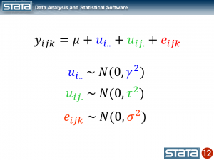
A good place to start is to simulate some multilevel RE data. Let’s create data for the 3-level regression model

where the classical multilevel regression assumption holds that and are distributed normal and are uncorrelated.

This represents a model of nested within nested within . An example would be students nested within schools nested within counties. We have random intercepts at the 2nd and 3rd levels — , . Because these are random effects, we need estimate only the variance of , , and .

For our simulated data, let’s assume there are 3 groups at the 3rd level, 2 groups at the 2nd level within each 3rd level group, and 2 individuals within each 2nd level group. Or, , , and . Having only 3 groups at the 3rd level is silly. It gives us only 3 observations to estimate the variance of . But with only observations, we will be able to easily see our entire dataset, and the concepts scale to any number of 3rd-level groups.

First, create our 3rd-level random effects — .

. set obs 3
. gen k = _n
. gen Uk = rnormal()

There are only 3 in our dataset.

I am showing the effects symbolically in the table rather than showing numeric values. It is the pattern of unique effects that will become interesting, not their actual values.

Now, create our 2nd-level random effects — — by doubling this data and creating 2nd-level effects.

. expand 2
. by k, sort: gen j = _n
. gen Vjk = rnormal()

We have 6 unique values of our 2nd-level effects and the same 3 unique values of our 3rd-level effects. Our original 3rd-level effects just appear twice each.

Now, create our 1st-level random effects — — which we typically just call errors.

. expand 2
. by k j, sort: gen i = _n
. gen Eijk = rnormal()

There are still only 3 unique in our dataset, and only 6 unique .

Finally, we create our regression data, using ,

. gen xijk = runiform()
. gen yijk = 2 * xijk + Uk + Vjk + Eijk

We could estimate our multilevel RE model on this data by typing,

. xtmixed yijk xijk || k: || j:

xtmixed uses the index variables k and j to deeply understand the multilevel structure of the our data. sem has no such understanding of multilevel data. What it does have is an understanding of multivariate data and a comfortable willingness to apply constraints.

Let’s restructure our data so that sem can be made to understand its multilevel structure.

First some renaming so that the results of our restructuring will be easier to interpret.

. rename Uk U
. rename Vjk V
. rename Eijk E
. rename xijk x
. rename yijk y

We reshape to turn our multilevel data into multivariate data that sem has a chance of understanding. First, we reshape wide on our 2nd-level identifier j. Before that, we egen to create a unique identifier for each observation of the two groups identified by j.

. egen ik = group(i k)
. reshape wide y x E V, i(ik) j(j)

We now have a y variable for each group in j (y1 and y2). Likewise, we have two x variables, two residuals, and most importantly two 2nd-level random effects V1 and V2. This is the same data, we have merely created a set of variables for every level of j. We have gone from multilevel to multivariate.
We still have a multilevel component. There are still two levels of i in our dataset. We must reshape wide again to remove any remnant of multilevel structure.

. drop ik
. reshape wide y* x* E*, i(k) j(i)

I admit that is a microscopic font, but it is the structure that is important, not the values. We now have 4 y’s, one for each combination of 2nd- and 3rd-level identifiers — i and j. Likewise for the x’s and E’s.

We can think of each xji yji pair of columns as representing a regression for a specific combination of j and i — y11 on x11, y12 on x12, y21 on x21, and y22 on x22. Or, more explicitly,

So, rather than a univariate multilevel regression with 4 nested observation sets, () * (), we now have 4 regressions which are all related through and each of two pairs are related through . Oh, and all share the same coefficient . Oh, and the all have identical variances. Oh, and the also have identical variances. Luckily both the sem command and the SEM Builder (the GUI for sem) make setting constraints easy.

There is one other thing we haven’t addressed. xtmixed understands random effects. Does sem? Random effects are just unobserved (latent) variables and sem clearly understands those. So, yes, sem does understand random effects.

Many SEMers would represent this model in a path diagram by drawing.

There is a lot of information in that diagram. Each regression is represented by one of the x boxes being connected by a path to a y box. That each of the four paths is labeled with means that we have constrained the regressions to have the same coefficient. The y21 and y22 boxes also receive input from the random latent variable V2 (representing our 2nd-level random effects). The other two y boxes receive input from V1 (also our 2nd-level random effects). For this to match how xtmixed handles random effects, V1 and V2 must be constrained to have the same variance. This was done in the path diagram by “locking” them to have the same variance — S_v. To match xtmixed, each of the four residuals must also have the same variance — shown in the diagram as S_e. The residuals and random effect variables also have their paths constrained to 1. That is to say, they do not have coefficients.

We do not need any of the U, V, or E variables. We kept these only to make clear how the multilevel data was restructured to multivariate data. We might “follow the money” in a criminal investigation, but with simulated multilevel data is is best to “follow the effects”. Seeing how these effects were distributed in our reshaped data made it clear how they entered our multivariate model.

Just to prove that this all works, here are the results from a simulated dataset ( rather than the 3 that we have been using). The xtmixed results are,

. xtmixed yijk xijk || k: || j: , mle var

  (log omitted)

Mixed-effects ML regression                     Number of obs      =       400

-----------------------------------------------------------
                |   No. of       Observations per Group
 Group Variable |   Groups    Minimum    Average    Maximum
----------------+------------------------------------------
              k |      100          4        4.0          4
              j |      200          2        2.0          2
-----------------------------------------------------------

                                                Wald chi2(1)       =     61.84
Log likelihood = -768.96733                     Prob > chi2        =    0.0000

------------------------------------------------------------------------------
        yijk |      Coef.   Std. Err.      z    P>|z|     [95% Conf. Interval]
-------------+----------------------------------------------------------------
        xijk |   1.792529   .2279392     7.86   0.000     1.345776    2.239282
       _cons |    .460124   .2242677     2.05   0.040     .0205673    .8996807
------------------------------------------------------------------------------

------------------------------------------------------------------------------
  Random-effects Parameters  |   Estimate   Std. Err.     [95% Conf. Interval]
-----------------------------+------------------------------------------------
k: Identity                  |
                  var(_cons) |   2.469012   .5386108      1.610034    3.786268
-----------------------------+------------------------------------------------
j: Identity                  |
                  var(_cons) |   1.858889    .332251      1.309522    2.638725
-----------------------------+------------------------------------------------
               var(Residual) |   .9140237   .0915914      .7510369    1.112381
------------------------------------------------------------------------------
LR test vs. linear regression:       chi2(2) =   259.16   Prob > chi2 = 0.0000

Note: LR test is conservative and provided only for reference.

The sem results are,

sem (y11 <- x11@bx _cons@c V1@1 U@1)
    (y12 <- x12@bx _cons@c V1@1 U@1)
    (y21 <- x21@bx _cons@c V2@1 U@1)
    (y22 <- x22@bx _cons@c V2@1 U@1) ,
        covstruct(_lexog, diagonal) cov(_lexog*_oexog@0)  
        cov( V1@S_v V2@S_v  e.y11@S_e e.y12@S_e e.y21@S_e e.y22@S_e)
  
  (notes omitted)

Endogenous variables

Observed:  y11 y12 y21 y22

Exogenous variables

Observed:  x11 x12 x21 x22
Latent:    V1 U V2
  
  (iteration log omitted)

Structural equation model                       Number of obs      =       100
Estimation method  = ml
Log likelihood     = -826.63615
  
  (constraint listing omitted)
------------------------------------------------------------------------------
             |                 OIM             |      Coef.   Std. Err.      z    P>|z|     [95% Conf. Interval]
-------------+----------------------------------------------------------------
Structural   |  
  y11 <-     |
         x11 |   1.792529   .2356323     7.61   0.000     1.330698     2.25436
          V1 |          1   7.68e-17  1.3e+16   0.000            1           1
           U |          1   2.22e-18  4.5e+17   0.000            1           1
       _cons |    .460124    .226404     2.03   0.042     .0163802    .9038677
  -----------+----------------------------------------------------------------
  y12 <-     |
         x12 |   1.792529   .2356323     7.61   0.000     1.330698     2.25436
          V1 |          1   2.00e-22  5.0e+21   0.000            1           1
           U |          1   5.03e-17  2.0e+16   0.000            1           1
       _cons |    .460124    .226404     2.03   0.042     .0163802    .9038677
  -----------+----------------------------------------------------------------
  y21 <-     |
         x21 |   1.792529   .2356323     7.61   0.000     1.330698     2.25436
           U |          1   5.70e-46  1.8e+45   0.000            1           1
          V2 |          1   5.06e-45  2.0e+44   0.000            1           1
       _cons |    .460124    .226404     2.03   0.042     .0163802    .9038677
  -----------+----------------------------------------------------------------
  y22 <-     |
         x22 |   1.792529   .2356323     7.61   0.000     1.330698     2.25436
           U |          1  (constrained)
          V2 |          1  (constrained) 
       _cons |    .460124    .226404     2.03   0.042     .0163802    .9038677
-------------+----------------------------------------------------------------
Variance     |
       e.y11 |   .9140239    .091602                        .75102    1.112407
       e.y12 |   .9140239    .091602                        .75102    1.112407
       e.y21 |   .9140239    .091602                        .75102    1.112407
       e.y22 |   .9140239    .091602                        .75102    1.112407
          V1 |   1.858889   .3323379                      1.309402    2.638967
           U |   2.469011   .5386202                      1.610021    3.786296
          V2 |   1.858889   .3323379                      1.309402    2.638967
-------------+----------------------------------------------------------------
Covariance   |
  x11        |
          V1 |          0  (constrained)
           U |          0  (constrained)
          V2 |          0  (constrained)
  -----------+----------------------------------------------------------------
  x12        |
          V1 |          0  (constrained)
           U |          0  (constrained)
          V2 |          0  (constrained)
  -----------+----------------------------------------------------------------
  x21        |
          V1 |          0  (constrained)
           U |          0  (constrained)
          V2 |          0  (constrained)
  -----------+----------------------------------------------------------------
  x22        |
          V1 |          0  (constrained)
           U |          0  (constrained)
          V2 |          0  (constrained)
  -----------+----------------------------------------------------------------
  V1         |
           U |          0  (constrained)
          V2 |          0  (constrained)
  -----------+----------------------------------------------------------------
  U          |
          V2 |          0  (constrained)
------------------------------------------------------------------------------
LR test of model vs. saturated: chi2(25)  =     22.43, Prob > chi2 = 0.6110

And here is the path diagram after estimation.

The standard errors of the two estimation methods are asymptotically equivalent, but will differ in finite samples.

Sidenote: Those familiar with multilevel modeling will be wondering if sem can handle unbalanced data. That is to say a different number of observations or subgroups within groups. It can. Simply let reshape create missing values where it will and then add the method(mlmv) option to your sem command. mlmv stands for maximum likelihood with missing values. And, as strange as it may seem, with this option the multivariate sem representation and the multilevel xtmixed representations are the same.

Do we care?

You will have noticed that the sem command was, well, it was really long. (I wrote a little loop to get all the constraints right.) You will also have noticed that there is a lot of redundant output because our SEM model has so many constraints. Why would anyone go to all this trouble to do something that is so simple with xtmixed? The answer lies in all of those constraints. With sem we can relax any of those constraints we wish!

Relax the constraint that the V# have the same variance and you can introduce heteroskedasticity in the 2nd-level effects. That seems a little silly when there are only two levels, but imagine there were 10 levels.

Add a covariance between the V# and you introduce correlation between the groups in the 3rd level.

What’s more, the pattern of heteroskedasticity and correlation can be arbitrary. Here is our path diagram redrawn to represent children within schools within counties and increasing the number of groups in the 2nd level.

We have 5 counties at the 3rd level and two schools within each county at the 2nd level — for a total of 10 dimensions in our multivariate regression. The diagram does not change based on the number of children drawn from each school.

Our regression coefficients have been organized horizontally down the center of the diagram to allow room along the left and right for the random effects. Taken as a multilevel model, we have only a single covariate — x. Just to be clear, we could generalize this to multiple covariates by adding more boxes with covariates for each dependent variable in the diagram.

The labels are chosen carefully. The 3rd-level effects N1, N2, and N3 are for northern counties, and the remaining second level effects S1 and S2 are for southern counties. There is a separate dependent variable and associated error for each school. We have 4 public schools (pub1 pub2, pub3, and pub4); three private schools (prv1 prv2, and prv3); and 3 church-sponsored schools (chr1 chr2, and chr3).

The multivariate structure seen in the diagram makes it clear that we can relax some constraints that the multilevel model imposes. Because the sem representation of the model breaks the 2nd level effect into an effect for each county, we can apply a structure to the 2nd level effect. Consider the path diagram below.

We have correlated the effects for the 3 northern counties. We did this by drawing curved lines between the effects. We have also correlated the effects of the two southern counties. xtmixed does not allow these types of correlations. Had we wished, we could have constrained the correlations of the 3 northern counties to be the same.

We could also have allowed the northern and southern counties to have different variances. We did just that in the diagram below by constraining the northern counties variances to be N and the southern counties variances to be S.

In this diagram we have also correlated the errors for the 4 public schools. As drawn, each correlation is free to take on its own values, but we could just as easily constrain each public school to be equally correlated with all other public schools. Likewise, to keep the diagram readable, we did not correlate the private schools with each other or the church schools with each other. We could have done that.

There is one thing that xtmixed can do that sem cannot. It can put a structure on the residual correlations within the 2nd level groups. xtmixed has a special option, residuals(), for just this purpose.

With xtmixed and sem you get,

• robust and cluster-robust SEs
• survey data

With sem you also get

• endogenous covariates
• estimation by GMM
• missing data — MAR (also called missing on observables)
• heteroskedastic effects at any level
• correlated effects at any level
• easy score tests using estat scoretests
  • are the coefficients truly are the same across all equations/levels, whether effects?
  • are effects or sets of effects uncorrelated?
  • are effects within a grouping homoskedastic?
  • …

Whether you view this rethinking of multilevel random-effects models as multivariate structural equation models (SEMs) as interesting, or merely an academic exercise, depends on whether your model calls for any of the items in the second list.

Have you every wanted to make an “easy” calculation–say, after fitting a model–and gotten lost because you just weren’t sure where to find the degrees of freedom of the residual or the standard error of the coefficient? Have you ever been in the midst of constructing an “easy” calculation and was suddenly unsure just what e(df_r) really was? I have a solution.

It’s called Stata’s expression builder. You can get to it from the display dialog (Data->Other Utilities->Hand Calculator)

In the dialog, click the Create button to bring up the builder. Really, it doesn’t look like much:

I want to show you how to use this expression builder; if you’ll stick with me, it’ll be worth your time.

Let’s start over again and assume you are in the midst of an analysis, say,

. sysuse auto, clear
. regress price mpg length

Next invoke the expression builder by pulling down the menu Data->Other Utilities->Hand Calculator. Click Create. It looks like this:

Now click on the tree node icon (+) in front of “Estimation results” and then scroll down to see what’s underneath. You’ll see

Click on Scalars:

The middle box now contains the scalars stored in e(). N happens to be highlighted, but you could click on any of the scalars. If you look below the two boxes, you see the value of the e() scalar selected as well as its value and a short description. e(N) is 74 and is the “number of observations”.

It works the same way for all the other categories in the box on the left: Operators, Functions, Variables, Coefficients, Estimation results, Returned results, System parameters, Matrices, Macros, Scalars, Notes, and Characteristics. You simply click on the tree node icon (+), and the category expands to show what is available.

You have now mastered the expression builder!

Let’s try it out.

Say you want to verify that the p-value of the coefficient on mpg is correctly calculated by regress–which reports 0.052–or more likely, you want to verify that you know how it was calculated. You think the formula is

or, as an expression in Stata,

2*ttail(e(df_r), abs(_b[mpg]/_se[mpg]))

But I’m jumping ahead. You may not remember that _b[mpg] is the coefficient on variable mpg, or that _se[mpg] is its corresponding standard error, or that abs() is Stata’s absolute value function, or that e(df_r) is the residual degrees of freedom from the regression, or that ttail() is Stata’s Student’s t distribution function. We can build the above expression using the builder because all the components can be accessed through the builder. The ttail() and abs() functions are in the Functions category, the e(df_r) scalar is in the Estimation results category, and _b[mpg] and _se[mpg] are in the Coefficients category.

What’s nice about the builder is that not only are the item names listed but also a definition, syntax, and value are displayed when you click on an item. Having all this information in one place makes building a complex expression much easier.

Another example of when the expression builder comes in handy is when computing intraclass correlations after xtmixed. Consider a simple two-level model from Example 1 in [XT] xtmixed, which models weight trajectories of 48 pigs from 9 successive weeks:

. use http://www.stata-press.com/data/r12/pig
. xtmixed weight week || id:, variance

The intraclass correlation is a nonlinear function of variance components. In this example, the (residual) intraclass correlation is the ratio of the between-pig variance, var(_cons), to the total variance, between-pig variance plus residual (within-pig) variance, or var(_cons) + var(residual).

The xtmixed command does not store the estimates of variance components directly. Instead, it stores them as log standard deviations in e(b) such that _b[lns1_1_1:_cons] is the estimated log of between-pig standard deviation, and _b[lnsig_e:_cons] is the estimated log of residual (within-pig) standard deviation. So to compute the intraclass correlation, we must first transform log standard deviations to variances:

exp(2*_b[lns1_1_1:_cons])
exp(2*_b[lnsig_e:_cons])

The final expression for the intraclass correlation is then

exp(2*_b[lns1_1_1:_cons]) / (exp(2*_b[lns1_1_1:_cons])+exp(2*_b[lnsig_e:_cons]))

The problem is that few people remember that _b[lns1_1_1:_cons] is the estimated log of between-pig standard deviation. The few who do certainly do not want to type it. So use the expression builder as we do below:

In this case, we’re using the expression builder accessed from Stata’s nlcom dialog, which reports estimated nonlinear combinations along with their standard errors. Once we press OK here and in the nlcom dialog, we’ll see

. nlcom (exp(2*_b[lns1_1_1:_cons])/(exp(2*_b[lns1_1_1:_cons])+exp(2*_b[lnsig_e:_cons])))

  _nl_1:  exp(2*_b[lns1_1_1:_cons])/(exp(2*_b[lns1_1_1:_cons])+exp(2*_b[lnsig_e:_cons]))

------------------------------------------------------------------------------
      weight |      Coef.   Std. Err.      z    P>|z|     [95% Conf. Interval]
-------------+----------------------------------------------------------------
       _nl_1 |   .7717142   .0393959    19.59   0.000     .6944996    .8489288
------------------------------------------------------------------------------

The above could easily be extended to computing different types of intraclass correlations arising in higher-level random-effects models. The use of the expression builder for that becomes even more handy.

Some of our users have asked about the way predictions are computed after fitting their models with arima. Those users report that they cannot reproduce the complete set of forecasts manually when the model contains MA terms. They specifically refer that they are not able to get the exact values for the first few predicted periods. The reason for the difference between their manual results and the forecasts obtained with predict after arima is the way the starting values and the recursive predictions are computed. While Stata uses the Kalman filter to compute the forecasts based on the state space representation of the model, users reporting differences compute their forecasts with a different estimator that is based on the recursions derived from the ARIMA representation of the model. Both estimators are consistent but they produce slightly different results for the first few forecasting periods.

When using the postestimation command predict after fitting their MA(1) model with arima, some users claim that they should be able to reproduce the predictions with

where

However, the recursive formula for the Kalman filter prediction is based on the shrunk error (See section 13.3 in Hamilton (1993) for the complete derivation based on the state space representation):

where

: is the estimated variance of the white noise disturbance

: corresponds to the unconditional mean for the error term

Let’s use one of the datasets available from our website to fit a MA(1) model and compute the predictions based on the Kalman filter recursions formulated above:

** Predictions with Kalman Filter recursions (obtained with -predict- **
use http://www.stata-press.com/data/r12/lutkepohl, clear
arima dlinvestment, ma(1)
predict double yhat

** Coefficient estimates and sigma^2 from ereturn list **
scalar beta = _b[_cons]
scalar theta = [ARMA]_b[L1.ma]
scalar sigma2 = e(sigma)^2

** pt and shrinking factor for the first two observations**
generate double pt=sigma2 in 1/2
generate double sh_factor=(sigma2)/(sigma2+theta^2*pt) in 2

** Predicted series and errors for the first two observations **
generate double my_yhat = beta
generate double myehat = sh_factor*(dlinvestment - my_yhat) in 2

** Predictions with the Kalman filter recursions **
quietly {
    forvalues i = 3/91 {
        replace my_yhat = my_yhat + theta*l.myehat in `i'
        replace pt= (sigma2*theta^2*L.pt)/(sigma2+theta^2*L.pt) in `i'
        replace sh_factor=(sigma2)/(sigma2+theta^2*pt)          in `i'
        replace myehat=sh_factor*(dlinvestment - my_yhat)       in `i'
    }
}

List the first 10 predictions (yhat from predict and my_yhat from the manual computations):

. list qtr yhat my_yhat pt sh_factor in 1/10

     +--------------------------------------------------------+
     |    qtr        yhat     my_yhat          pt   sh_factor |
     |--------------------------------------------------------|
  1. | 1960q1   .01686688   .01686688   .00192542           . |
  2. | 1960q2   .01686688   .01686688   .00192542   .97272668 |
  3. | 1960q3   .02052151   .02052151   .00005251   .99923589 |
  4. | 1960q4   .01478403   .01478403   1.471e-06   .99997858 |
  5. | 1961q1   .01312365   .01312365   4.125e-08    .9999994 |
     |--------------------------------------------------------|
  6. | 1961q2   .00326376   .00326376   1.157e-09   .99999998 |
  7. | 1961q3   .02471242   .02471242   3.243e-11           1 |
  8. | 1961q4   .01691061   .01691061   9.092e-13           1 |
  9. | 1962q1   .01412974   .01412974   2.549e-14           1 |
 10. | 1962q2   .00643301   .00643301   7.147e-16           1 |
     +--------------------------------------------------------+

Notice that the shrinking factor (sh_factor) tends to 1 as t increases, which implies that after a few initial periods the predictions produced with the Kalman filter recursions become exactly the same as the ones produced by the formula at the top of this entry for the recursions derived from the ARIMA representation of the model.

Reference:

Hamilton, James. 1994. Time Series Analysis. Princeton University Press.

I just got back from the 2012 Stata Conference in San Diego where I gave a talk on Psychometric Analysis Using Stata and from the 2012 American Psychological Association Meeting in Orlando. Stata’s structural equation modeling (SEM) builder was popular at both meetings and I wanted to show you how easy it is to use. If you are not familiar with the basics of SEM, please refer to the references at the end of the blog. My goal is simply to show you how to use the SEM builder assuming that you already know something about SEM. If you would like to view a video demonstration of the SEM builder, please click the play button below:

The data used here and for the silly examples in my talk were simulated to resemble one of the most commonly used measures of depression: the Beck Depression Inventory (BDI). If you find these data too silly or not relevant to your own research, you could instead imagine it being a set of questions to measure mathematical ability, the ability to use a statistical package, or whatever you wanted.

The Beck Depression Inventory

Originally published by Aaron Beck and colleagues in 1961, the BDI marked an important change in the conceptualization of depression from a psychoanalytic perspective to a cognitive/behavioral perspective. It was also a landmark in the measurement of depression shifting from lengthy, expensive interviews with a psychiatrist to a brief, inexpensive questionnaire that could be scored and quantified. The original inventory consisted of 21 questions each allowing ordinal responses of increasing symptom severity from 0-3. The sum of the responses could then be used to classify a respondent’s depressive symptoms as none, mild, moderate or severe. Many studies have demonstrated that the BDI has good psychometric properties such as high test-retest reliability and the scores correlate well with the assessments of psychiatrists and psychologists. The 21 questions can also be grouped into two subscales. The affective scale includes questions like “I feel sad” and “I feel like a failure” that quantify emotional symptoms of depression. The somatic or physical scale includes questions like “I have lost my appetite” and “I have trouble sleeping” that quantify physical symptoms of depression. Since its original publication, the BDI has undergone two revisions in response to the American Psychiatric Association’s (APA) Diagnostic and Statistical Manuals (DSM) and the BDI-II remains very popular.

The Stata Depression Inventory

Since the BDI is a copyrighted psychometric instrument, I created a fictitious instrument called the “Stata Depression Inventory”. It consists of 20 questions each beginning with the phrase “My statistical software makes me…”. The individual questions are listed in the variable labels below.

. describe qu1-qu20

variable  storage  display    value
 name       type   format     label      variable label
------------------------------------------------------------------------------
qu1         byte   %16.0g     response   ...feel sad
qu2         byte   %16.0g     response   ...feel pessimistic about the future
qu3         byte   %16.0g     response   ...feel like a failure
qu4         byte   %16.0g     response   ...feel dissatisfied
qu5         byte   %16.0g     response   ...feel guilty or unworthy
qu6         byte   %16.0g     response   ...feel that I am being punished
qu7         byte   %16.0g     response   ...feel disappointed in myself
qu8         byte   %16.0g     response   ...feel am very critical of myself
qu9         byte   %16.0g     response   ...feel like harming myself
qu10        byte   %16.0g     response   ...feel like crying more than usual
qu11        byte   %16.0g     response   ...become annoyed or irritated easily
qu12        byte   %16.0g     response   ...have lost interest in other people
qu13        byte   %16.0g     qu13_t1    ...have trouble making decisions
qu14        byte   %16.0g     qu14_t1    ...feel unattractive
qu15        byte   %16.0g     qu15_t1    ...feel like not working
qu16        byte   %16.0g     qu16_t1    ...have trouble sleeping
qu17        byte   %16.0g     qu17_t1    ...feel tired or fatigued
qu18        byte   %16.0g     qu18_t1    ...makes my appetite lower than usual
qu19        byte   %16.0g     qu19_t1    ...concerned about my health
qu20        byte   %16.0g     qu20_t1    ...experience decreased libido

The responses consist of a 5-point Likert scale ranging from 1 (Strongly Disagree) to 5 (Strongly Agree). Questions 1-10 form the affective scale of the inventory and questions 11-20 form the physical scale. Data were simulated for 1000 imaginary people and included demographic variables such as age, sex and race. The responses can be summarized succinctly in a matrix of bar graphs:

Classical statistical analysis

The beginning of a classical statistical analysis of these data might consist of summing the responses for questions 1-10 and referring to them as the “Affective Depression Score” and summing questions 11-20 and referring to them as the “Physical Depression Score”.

egen Affective = rowtotal(qu1-qu10)
label var Affective "Affective Depression Score"
egen physical = rowtotal(qu11-qu20)
label var physical "Physical Depression Score"

We could be more sophisticated and use principal components to create the affective and physical depression score:

pca qu1-qu20, components(2)
predict Affective Physical
label var Affective "Affective Depression Score"
label var Physical "Physical Depression Score"

We could then ask questions such as “Are there differences in affective and physical depression scores by sex?” and test these hypotheses using multivariate statistics such as Hotelling’s T-squared statistic. The problem with this analysis strategy is that it treats the depression scores as though they were measured without error and can lead to inaccurate p-values for our test statistics.

Structural equation modeling

Structural equation modeling (SEM) is an ideal way to analyze data where the outcome of interest is a scale or scales derived from a set of measured variables. The affective and physical scores are treated as latent variables in the model resulting in accurate p-values and, best of all….these models are very easy to fit using Stata! We begin by selecting the SEM builder from the Statistics menu:

In the SEM builder, we can select the “Add Measurement Component” icon:

which will open the following dialog box:

In the box labeled “Latent Variable Name” we can type “Affective” (red arrow below) and we can select the variables qu1-qu10 in the “Measured variables” box (blue arrow below).

When we click “OK”, the affective measurement component appears in the builder:

We can repeat this process to create a measurement component for our physical depression scale (images not shown). We can also allow for covariance/correlation between our affective and physical depression scales using the “Add Covariance” icon on the toolbar (red arrow below).

I’ll omit the intermediate steps to build the full model shown below but it’s easy to use the “Add Observed Variable” and “Add Path” icons to create the full model:

Now we’re ready to estimate the parameters for our model. To do this, we click the “Estimate” icon on the toolbar (duh!):

And the flowing dialog box appears:

Let’s ignore the estimation options for now and use the default settings. Click “OK” and the parameter estimates will appear in the diagram:

Some of the parameter estimates are difficult to read in this form but it is easy to rearrange the placement and formatting of the estimates to make them easier to read.

If we look at Stata’s output window and scroll up, you’ll notice that the SEM Builder automatically generated the command for our model:

sem (Affective -> qu1) (Affective -> qu2) (Affective -> qu3)
    (Affective -> qu4) (Affective -> qu5) (Affective -> qu6)
    (Affective -> qu7) (Affective -> qu8) (Affective -> qu9)
    (Affective -> qu10) (Physical -> qu11) (Physical -> qu12)
    (Physical -> qu13) (Physical -> qu14) (Physical -> qu15)
    (Physical -> qu16) (Physical -> qu17) (Physical -> qu18)
    (Physical -> qu19) (Physical -> qu20) (sex -> Affective)
    (sex -> Physical), latent(Affective Physical) cov(e.Physical*e.Affective)

We can gather terms and abbreviate some things to make the command much easier to read:

sem (Affective -> qu1-qu10) ///
    (Physical -> qu11-qu20) /// 
    (sex -> Affective Physical) ///
    , latent(Affective Physical ) ///
    cov( e.Physical*e.Affective)

We could then calculate a Wald statistic to test the null hypothesis that there is no association between sex and our affective and physical depression scales.

test sex

 ( 1)  [Affective]sex = 0
 ( 2)  [Physical]sex = 0

           chi2(  2) =    2.51
         Prob > chi2 =    0.2854

Final thoughts
This is an admittedly oversimplified example – we haven’t considered the fit of the model or considered any alternative models. We have only included one dichotomous independent variable. We might prefer to use a likelihood ratio test or a score test. Those are all very important issues and should not be ignored in a proper data analysis. But my goal was to demonstrate how easy it is to use Stata’s SEM builder to model data such as those arising from the Beck Depression Inventory. Incidentally, if these data were collected using a complex survey design, it would not be difficult to incorporate the sampling structure and sample weights into the analysis. Missing data can be handled easily as well using Full Information Maximum Likelihood (FIML) but those are topics for another day.

If you would like view the slides from my talk, download the data used in this example or view a video demonstration of Stata’s SEM builder using these data, please use the links below. For the dataset, you can also type use followed by the URL for the data to load it directly into Stata.

Slides:
http://stata.com/meeting/sandiego12/materials/sd12_huber.pdf

Data:
http://stata.com/meeting/sandiego12/materials/Huber_2012SanDiego.dta

YouTube video demonstration:
http://www.youtube.com/watch?v=Xj0gBlqwYHI

References

Beck AT, Ward CH, Mendelson M, Mock J, Erbaugh J (June 1961). An inventory for measuring depression. Arch. Gen. Psychiatry 4 (6): 561–71.

Beck AT, Ward C, Mendelson M (1961). Beck Depression Inventory (BDI). Arch Gen Psychiatry 4 (6): 561–571

Beck AT, Steer RA, Ball R, Ranieri W (December 1996). Comparison of Beck Depression Inventories -IA and -II in psychiatric outpatients. Journal of Personality Assessment 67 (3): 588–97
Bollen, KA. (1989). Structural Equations With Latent Variables. New York, NY: John Wiley and Sons

Kline, RB (2011). Principles and Practice of Structural Equation Modeling. New York, NY: Guilford Press

Raykov, T & Marcoulides, GA (2006). A First Course in Structural Equation Modeling. Mahwah, NJ: Lawrence Erlbaum

Schumacker, RE & Lomax, RG (2012) A Beginner’s Guide to Structural Equation Modeling, 3rd Ed. New York, NY: Routledge

In the last 15-20 years multilevel modeling has evolved from a specialty area of statistical research into a standard analytical tool used by many applied researchers.

Stata has a lot of multilevel modeling capababilities.

I want to show you how easy it is to fit multilevel models in Stata. Along the way, we’ll unavoidably introduce some of the jargon of multilevel modeling.

I’m going to focus on concepts and ignore many of the details that would be part of a formal data analysis. I’ll give you some suggestions for learning more at the end of the blog.

The videos

Stata has a friendly dialog box that can assist you in building multilevel models. If you would like a brief introduction using the GUI, you can watch a demonstration on Stata’s YouTube Channel:

Introduction to multilevel linear models in Stata, part 1: The xtmixed command

Multilevel data

Multilevel data are characterized by a hierarchical structure. A classic example is children nested within classrooms and classrooms nested within schools. The test scores of students within the same classroom may be correlated due to exposure to the same teacher or textbook. Likewise, the average test scores of classes might be correlated within a school due to the similar socioeconomic level of the students.

You may have run across datasets with these kinds of structures in your own work. For our example, I would like to use a dataset that has both longitudinal and classical hierarchical features. You can access this dataset from within Stata by typing the following command:

use http://www.stata-press.com/data/r12/productivity.dta

We are going to build a model of gross state product for 48 states in the USA measured annually from 1970 to 1986. The states have been grouped into nine regions based on their economic similarity. For distributional reasons, we will be modeling the logarithm of annual Gross State Product (GSP) but in the interest of readability, I will simply refer to the dependent variable as GSP.

. describe gsp year state region

              storage  display     value
variable name   type   format      label      variable label
-----------------------------------------------------------------------------
gsp             float  %9.0g                  log(gross state product)
year            int    %9.0g                  years 1970-1986
state           byte   %9.0g                  states 1-48
region          byte   %9.0g                  regions 1-9

Let’s look at a graph of these data to see what we’re working with.

twoway (line gsp year, connect(ascending)), ///
        by(region, title("log(Gross State Product) by Region", size(medsmall)))

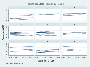
Each line represents the trajectory of a state’s (log) GSP over the years 1970 to 1986. The first thing I notice is that the groups of lines are different in each of the nine regions. Some groups of lines seem higher and some groups seem lower. The second thing that I notice is that the slopes of the lines are not the same. I’d like to incorporate those attributes of the data into my model.

Components of variance

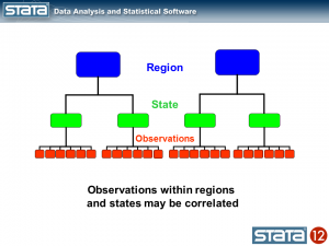
Let’s tackle the vertical differences in the groups of lines first. If we think about the hierarchical structure of these data, I have repeated observations nested within states which are in turn nested within regions. I used color to keep track of the data hierarchy.

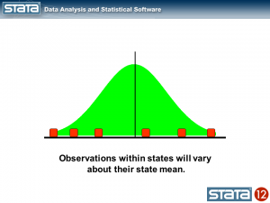
We could compute the mean GSP within each state and note that the observations within in each state vary about their state mean.

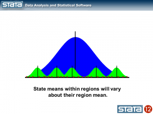
Likewise, we could compute the mean GSP within each region and note that the state means vary about their regional mean.

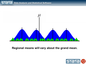
We could also compute a grand mean and note that the regional means vary about the grand mean.

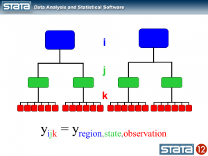
Next, let’s introduce some notation to help us keep track of our mutlilevel structure. In the jargon of multilevel modelling, the repeated measurements of GSP are described as “level 1″, the states are referred to as “level 2″ and the regions are “level 3″. I can add a three-part subscript to each observation to keep track of its place in the hierarchy.

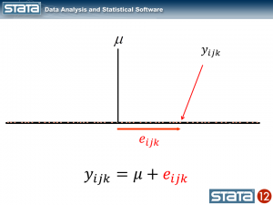
Now let’s think about our model. The simplest regression model is the intercept-only model which is equivalent to the sample mean. The sample mean is the “fixed” part of the model and the difference between the observation and the mean is the residual or “random” part of the model. Econometricians often prefer the term “disturbance”. I’m going to use the symbol μ to denote the fixed part of the model. μ could represent something as simple as the sample mean or it could represent a collection of independent variables and their parameters.

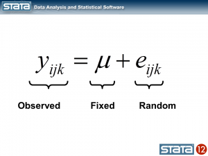
Each observation can then be described in terms of its deviation from the fixed part of the model.

If we computed this deviation of each observation, we could estimate the variability of those deviations. Let’s try that for our data using Stata’s xtmixed command to fit the model:

. xtmixed gsp

Mixed-effects ML regression                     Number of obs      =       816

                                                Wald chi2(0)       =         .
Log likelihood = -1174.4175                     Prob > chi2        =         .

------------------------------------------------------------------------------
         gsp |      Coef.   Std. Err.      z    P>|z|     [95% Conf. Interval]
-------------+----------------------------------------------------------------
       _cons |   10.50885   .0357249   294.16   0.000     10.43883    10.57887
------------------------------------------------------------------------------

------------------------------------------------------------------------------
  Random-effects Parameters  |   Estimate   Std. Err.     [95% Conf. Interval]
-----------------------------+------------------------------------------------
                sd(Residual) |   1.020506   .0252613      .9721766    1.071238
------------------------------------------------------------------------------

The top table in the output shows the fixed part of the model which looks like any other regression output from Stata, and the bottom table displays the random part of the model. Let’s look at a graph of our model along with the raw data and interpret our results.

predict GrandMean, xb
label var GrandMean "GrandMean"
twoway  (line GrandMean year, lcolor(black) lwidth(thick))              ///
        (scatter gsp year, mcolor(red) msize(tiny)),                    ///
        ytitle(log(Gross State Product), margin(medsmall))              ///
        legend(cols(4) size(small))                                     ///
        title("GSP for 1970-1986 by Region", size(medsmall))

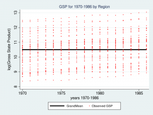
The thick black line in the center of the graph is the estimate of _cons, which is an estimate of the fixed part of model for GSP. In this simple model, _cons is the sample mean which is equal to 10.51. In “Random-effects Parameters” section of the output, sd(Residual) is the average vertical distance between each observation (the red dots) and fixed part of the model (the black line). In this model, sd(Residual) is the estimate of the sample standard deviation which equals 1.02.

At this point you may be thinking to yourself – “That’s not very interesting – I could have done that with Stata’s summarize command”. And you would be correct.

. summ gsp

    Variable |       Obs        Mean    Std. Dev.       Min        Max
-------------+--------------------------------------------------------
         gsp |       816    10.50885    1.021132    8.37885   13.04882

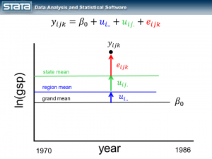
But here’s where it does become interesting. Let’s make the random part of the model more complex to account for the hierarchical structure of the data. Consider a single observation, y_ijk and take another look at its residual.

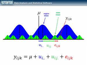
The observation deviates from its state mean by an amount that we will denote e_ijk. The observation’s state mean deviates from the the regionals mean u_ij. and the observation’s regional mean deviates from the fixed part of the model, μ, by an amount that we will denote u_i... We have partitioned the observation’s residual into three parts, aka “components”, that describe its magnitude relative to the state, region and grand means. If we calculated this set of residuals for each observation, wecould estimate the variability of those residuals and make distributional assumptions about them.

These kinds of models are often called “variance component” models because they estimate the variability accounted for by each level of the hierarchy. We can estimate a variance component model for GSP using Stata’s xtmixed command:

xtmixed gsp, || region: || state:

------------------------------------------------------------------------------
         gsp |      Coef.   Std. Err.      z    P>|z|     [95% Conf. Interval]
-------------+----------------------------------------------------------------
       _cons |   10.65961   .2503806    42.57   0.000     10.16887    11.15035
------------------------------------------------------------------------------

------------------------------------------------------------------------------
  Random-effects Parameters  |   Estimate   Std. Err.     [95% Conf. Interval]
-----------------------------+------------------------------------------------
region: Identity             |   
                   sd(_cons) |   .6615227   .2038944       .361566    1.210325
-----------------------------+------------------------------------------------
state: Identity              |   
                   sd(_cons) |   .7797837   .0886614      .6240114    .9744415
-----------------------------+------------------------------------------------
                sd(Residual) |   .1570457   .0040071       .149385    .1650992
------------------------------------------------------------------------------

The fixed part of the model, _cons, is still the sample mean. But now there are three parameters estimates in the bottom table labeled “Random-effects Parameters”. Each quantifies the average deviation at each level of the hierarchy.

Let’s graph the predictions from our model and see how well they fit the data.

predict GrandMean, xb
label var GrandMean "GrandMean"
predict RegionEffect, reffects level(region)
predict StateEffect, reffects level(state)
gen RegionMean = GrandMean + RegionEffect
gen StateMean = GrandMean + RegionEffect + StateEffect

twoway  (line GrandMean year, lcolor(black) lwidth(thick))      ///
        (line RegionMean year, lcolor(blue) lwidth(medthick))   ///
        (line StateMean year, lcolor(green) connect(ascending)) ///
        (scatter gsp year, mcolor(red) msize(tiny)),            ///
        ytitle(log(Gross State Product), margin(medsmall))      ///
        legend(cols(4) size(small))                             ///
        by(region, title("Multilevel Model of GSP by Region", size(medsmall)))

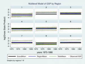
Wow – that’s a nice graph if I do say so myself. It would be impressive for a report or publication, but it’s a little tough to read with all nine regions displayed at once. Let’s take a closer look at Region 7 instead.

twoway  (line GrandMean year, lcolor(black) lwidth(thick))      ///
        (line RegionMean year, lcolor(blue) lwidth(medthick))   ///
        (line StateMean year, lcolor(green) connect(ascending)) ///
        (scatter gsp year, mcolor(red) msize(medsmall))         ///
        if region ==7,                                          ///
        ytitle(log(Gross State Product), margin(medsmall))      ///
        legend(cols(4) size(small))                             ///
        title("Multilevel Model of GSP for Region 7", size(medsmall))

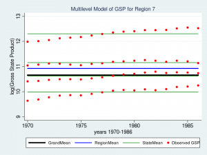
The red dots are the observations of GSP for each state within Region 7. The green lines are the estimated mean GSP within each State and the blue line is the estimated mean GSP within Region 7. The thick black line in the center is the overall grand mean for all nine regions. The model appears to fit the data fairly well but I can’t help noticing that the red dots seem to have an upward slant to them. Our model predicts that GSP is constant within each state and region from 1970 to 1986 when clearly the data show an upward trend.

So we’ve tackled the first feature of our data. We’ve succesfully incorporated the basic hierarchical structure into our model by fitting a variance componentis using Stata’s xtmixed command. But our graph tells us that we aren’t finished yet.

Next time we’ll tackle the second feature of our data — the longitudinal nature of the observations.

For more information

If you’d like to learn more about modelling multilevel and longitudinal data, check out

Multilevel and Longitudinal Modeling Using Stata, Third Edition
Volume I: Continuous Responses
Volume II: Categorical Responses, Counts, and Survival
by Sophia Rabe-Hesketh and Anders Skrondal

or sign up for our popular public training course “Multilevel/Mixed Models Using Stata“.

There’s a course coming up in Washington, DC on February 7-8, 2013.

In my last posting, I introduced you to the concepts of hierarchical or “multilevel” data. In today’s blog, I’d like to show you how to use multilevel modeling techniques to analyse longitudinal data with Stata’s xtmixed command.

Last time, we noticed that our data had two features. First, we noticed that the means within each level of the hierarchy were different from each other and we incorporated that into our data analysis by fitting a “variance component” model using Stata’s xtmixed command.

The second feature that we noticed is that repeated measurement of GSP showed an upward trend. We’ll pick up where we left off last time and stick to the concepts again and you can refer to the references at the end to learn more about the details.

The videos

Stata has a very friendly dialog box that can assist you in building multilevel models. If you would like a brief introduction using the GUI, you can watch a demonstration on Stata’s YouTube Channel:

Introduction to multilevel linear models in Stata, part 2: Longitudinal data

Longitudinal data

I’m often asked by beginning data analysts – “What’s the difference between longitudinal data and time-series data? Aren’t they the same thing?”.

The confusion is understandable — both types of data involve some measurement of time. But the answer is no, they are not the same thing.

Univariate time series data typically arise from the collection of many data points over time from a single source, such as from a person, country, financial instrument, etc.

Longitudinal data typically arise from collecting a few observations over time from many sources, such as a few blood pressure measurements from many people.

There are some multivariate time series that blur this distinction but a rule of thumb for distinguishing between the two is that time series have more repeated observations than subjects while longitudinal data have more subjects than repeated observations.

Because our GSP data from last time involve 17 measurements from 48 states (more sources than measurements), we will treat them as longitudinal data.

GSP Data: http://www.stata-press.com/data/r12/productivity.dta

Random intercept models

As I mentioned last time, repeated observations on a group of individuals can be conceptualized as multilevel data and modeled just as any other multilevel data. We left off last time with a variance component model for GSP (Gross State Product, logged) and noted that our model assumed a constant GSP over time while the data showed a clear upward trend.

If we consider a single observation and think about our model, nothing in the fixed or random part of the models is a function of time.

Let’s begin by adding the variable year to the fixed part of our model.

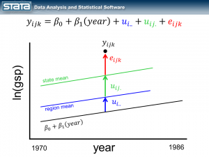
As we expected, our grand mean has become a linear regression which more accurately reflects the change over time in GSP. What might be unexpected is that each state’s and region’s mean has changed as well and now has the same slope as the regression line. This is because none of the random components of our model are a function of time. Let’s fit this model with the xtmixed command:

. xtmixed gsp year, || region: || state:

------------------------------------------------------------------------------
         gsp |      Coef.   Std. Err.      z    P>|z|     [95% Conf. Interval]
-------------+----------------------------------------------------------------
        year |   .0274903   .0005247    52.39   0.000     .0264618    .0285188
       _cons |  -43.71617   1.067718   -40.94   0.000    -45.80886   -41.62348
------------------------------------------------------------------------------

------------------------------------------------------------------------------
  Random-effects Parameters  |   Estimate   Std. Err.     [95% Conf. Interval]
-----------------------------+------------------------------------------------
region: Identity             |
                   sd(_cons) |   .6615238   .2038949      .3615664    1.210327
-----------------------------+------------------------------------------------
state: Identity              |
                   sd(_cons) |   .7805107   .0885788      .6248525    .9749452
-----------------------------+------------------------------------------------
                sd(Residual) |   .0734343   .0018737      .0698522    .0772001
------------------------------------------------------------------------------

The fixed part of our model now displays an estimate of the intercept (_cons = -43.7) and the slope (year = 0.027). Let’s graph the model for Region 7 and see if it fits the data better than the variance component model.

predict GrandMean, xb
label var GrandMean "GrandMean"
predict RegionEffect, reffects level(region)
predict StateEffect, reffects level(state)
gen RegionMean = GrandMean + RegionEffect
gen StateMean = GrandMean + RegionEffect + StateEffect

twoway  (line GrandMean year, lcolor(black) lwidth(thick))      ///
        (line RegionMean year, lcolor(blue) lwidth(medthick))   ///
        (line StateMean year, lcolor(green) connect(ascending)) ///
        (scatter gsp year, mcolor(red) msize(medsmall))         ///
        if region ==7,                                          ///
        ytitle(log(Gross State Product), margin(medsmall))      ///
        legend(cols(4) size(small))                             ///
        title("Multilevel Model of GSP for Region 7", size(medsmall))

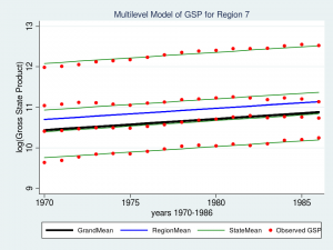
That looks like a much better fit than our variance-components model from last time. Perhaps I should leave well enough alone, but I can’t help noticing that the slopes of the green lines for each state don’t fit as well as they could. The top green line fits nicely but the second from the top looks like it slopes upward more than is necessary. That’s the best fit we can achieve if the regression lines are forced to be parallel to each other. But what if the lines were not forced to be parallel? What if we could fit a “mini-regression model” for each state within the context of my overall multilevel model. Well, good news — we can!

Random slope models

By introducing the variable year to the fixed part of the model, we turned our grand mean into a regression line. Next I’d like to incorporate the variable year into the random part of the model. By introducing a fourth random component that is a function of time, I am effectively estimating a separate regression line within each state.

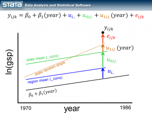
Notice that the size of the new, brown deviation u_1ij. is a function of time. If the observation were one year to the left, u_1ij. would be smaller and if the observation were one year to the right, u_1ij.would be larger.

It is common to “center” the time variable before fitting these kinds of models. Explaining why is for another day. The quick answer is that, at some point during the fitting of the model, Stata will have to compute the equivalent of the inverse of the square of year. For the year 1986 this turns out to be 2.535e-07. That’s a fairly small number and if we multiply it by another small number…well, you get the idea. By centering age (e.g. cyear = year – 1978), we get a more reasonable number for 1986 (0.01). (Hint: If you have problems with your model converging and you have large values for time, try centering them. It won’t always help, but it might).

So let’s center our year variable by subtracting 1978 and fit a model that includes a random slope.

gen cyear = year - 1978
xtmixed gsp cyear, || region: || state: cyear, cov(indep)

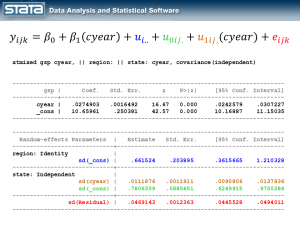
I’ve color-coded the output so that we can match each part of the output back to the model and the graph. The fixed part of the model appears in the top table and it looks like any other simple linear regression model. The random part of the model is definitely more complicated. If you get lost, look back at the graphic of the deviations and remind yourself that we have simply partitioned the deviation of each observation into four components. If we did this for every observation, the standard deviations in our output are simply the average of those deviations.

Let’s look at a graph of our new “random slope” model for Region 7 and see how well it fits our data.

predict GrandMean, xb
label var GrandMean "GrandMean"
predict RegionEffect, reffects level(region)
predict StateEffect_year StateEffect_cons, reffects level(state)

gen RegionMean = GrandMean + RegionEffect
gen StateMean_cons = GrandMean + RegionEffect + StateEffect_cons
gen StateMean_year = GrandMean + RegionEffect + StateEffect_cons + ///
                     (cyear*StateEffect_year)

twoway  (line GrandMean cyear, lcolor(black) lwidth(thick))             ///
        (line RegionMean cyear, lcolor(blue) lwidth(medthick))          ///
        (line StateMean_cons cyear, lcolor(green) connect(ascending))   ///
        (line StateMean_year cyear, lcolor(brown) connect(ascending))   ///
        (scatter gsp cyear, mcolor(red) msize(medsmall))                ///
        if region ==7,                                                  ///
        ytitle(log(Gross State Product), margin(medsmall))              ///
        legend(cols(3) size(small))                                     ///
        title("Multilevel Model of GSP for Region 7", size(medsmall))

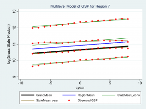
The top brown line fits the data slightly better, but the brown line below it (second from the top) is a much better fit. Mission accomplished!

Where do we go from here?

I hope I have been able to convince you that multilevel modeling is easy using Stata’s xtmixed command and that this is a tool that you will want to add to your kit. I would love to say something like “And that’s all there is to it. Go forth and build models!”, but I would be remiss if I didn’t point out that I have glossed over many critical topics.

In our GSP example, we would still like to consider the impact of other independent variables. I haven’t mentioned choice of estimation methods (ML or REML in the case of xtmixed). I’ve assessed the fit of our models by looking at graphs, an approach important but incomplete. We haven’t thought about hypothesis testing. Oh — and, all the usual residual diagnostics for linear regression such as checking for outliers, influential observations, heteroskedasticity and normality still apply….times four! But now that you understand the concepts and some of the mechanics, it shouldn’t be difficult to fill in the details. If you’d like to learn more, check out the links below.

I hope this was helpful…thanks for stopping by.

For more information

If you’d like to learn more about modeling multilevel and longitudinal data, check out

Multilevel and Longitudinal Modeling Using Stata, Third Edition
Volume I: Continuous Responses
Volume II: Categorical Responses, Counts, and Survival
by Sophia Rabe-Hesketh and Anders Skrondal

or sign up for our popular public training course Multilevel/Mixed Models Using Stata.

Today I want to talk about effect sizes such as Cohen’s d, Hedges’s g, Glass’s Δ, η², and ω². Effects sizes concern rescaling parameter estimates to make them easier to interpret, especially in terms of practical significance.

Many researchers in psychology and education advocate reporting of effect sizes, professional organizations such as the American Psychological Association (APA) and the American Educational Research Association (AERA) strongly recommend their reporting, and professional journals such as the Journal of Experimental Psychology: Applied and Educational and Psychological Measurement require that they be reported.

Anyway, today I want to show you

1. What effect sizes are.
2. How to calculate effect sizes and their confidence intervals in Stata.
3. How to calculate bootstrap confidence intervals for those effect sizes.
4. How to use Stata’s effect-size calculator.

1. What are effect sizes?

The importance of research results is often assessed by statistical significance, usually that the p-value is less than 0.05. P-values and statistical significance, however, don’t tell us anything about practical significance.

What if I told you that I had developed a new weight-loss pill and that the difference between the average weight loss for people who took the pill and the those who took a placebo was statistically significant? Would you buy my new pill? If you were overweight, you might reply, “Of course! I’ll take two bottles and a large order of french fries to go!”. Now let me add that the average difference in weight loss was only one pound over the year. Still interested? My results may be statistically significant but they are not practically significant.

Or what if I told you that the difference in weight loss was not statistically significant — the p-value was “only” 0.06 — but the average difference over the year was 20 pounds? You might very well be interested in that pill.

The size of the effect tells us about the practical significance. P-values do not assess practical significance.

All of which is to say, one should report parameter estimates along with statistical significance.

In my examples above, you knew that 1 pound over the year is small and 20 pounds is large because you are familiar with human weights.

In another context, 1 pound might be large, and in yet another, 20 pounds small.

Formal measures of effects sizes are thus usually presented in unit-free but easy-to-interpret form, such as standardized differences and proportions of variability explained.

The “d” family

Effect sizes that measure the scaled difference between means belong to the “d” family. The generic formula is

The estimators differ in terms of how sigma is calculated.

Cohen’s d, for instance, uses the pooled sample standard deviation.

Hedges’s g incorporates an adjustment which removes the bias of Cohen’s d.

Glass’s Δ was originally developed in the context of experiments and uses the “control group” standard deviation in the denominator. It has subsequently been generalized to nonexperimental studies. Because there is no control group in observational studies, Kline (2013) recommends reporting Glass’s Δ using the standard deviation for each group. Glass’s Delta_1 uses one group’s standard deviation and Delta_2 uses the other group’s.

Although I have given definitions to Cohen’s d, Hedges’s g, and Glass’s Δ, different authors swap the definitions around! As a result, many authors refer to all of the above as just Delta.

Be careful when using software to know which Delta you are getting. I have used Stata terminology, of course.

Anyway, the use of a standardized scale allows us to assess of practical significance. Delta = 1.5 indicates that the mean of one group is 1.5 standard deviations higher than that of the other. A difference of 1.5 standard deviations is obviously large, and a difference of 0.1 standard deviations is obviously small.

The “r” family

The r family quantifies the ratio of the variance attributable to an effect to the total variance and is often interpreted as the “proportion of variance explained”. The generic estimator is known as eta-squared,

η² is equivalent to the R-squared statistic from linear regression.

ω² is a less biased variation of η² that is equivalent to the adjusted R-squared.

Both of these measures concern the entire model.

Partial η² and partial ω² are like partial R-squareds and concern individual terms in the model. A term might be a variable or a variable and its interaction with another variable.

Both the d and r families allow us to make an apples-to-apples comparison of variables measured on different scales. For example, an intervention could affect both systolic blood pressure and total cholesterol. Comparing the relative effect of the intervention on the two outcomes would be difficult on their original scales.

How does one compare mm/Hg and mg/dL? It is straightforward in terms of Cohen’s d or ω² because then we are comparing standard deviation changes or proportion of variance explained.

2. How to calculate effect sizes and their confidence intervals in Stata

Consider a study where 30 school children are randomly assigned to classrooms that incorporated web-based instruction (treatment) or standard classroom environments (control). At the end of the school year, the children were given tests to measure reading and mathematics skills. The reading test is scored on a 0-15 point scale and, the mathematics test, on a 0-100 point scale.

Let’s download a dataset for our fictitious example from the Stata website by typing:

. use http://www.stata.com/videos13/data/webclass.dta

Contains data from http://www.stata.com/videos13/data/webclass.dta
  obs:            30                          Fictitious web-based learning 
                                                experiment data
 vars:             5                          5 Sep 2013 11:28
 size:           330                          (_dta has notes)
-------------------------------------------------------------------------------
              storage   display    value
variable name   type    format     label      variable label
-------------------------------------------------------------------------------
id              byte    %9.0g                 ID Number
treated         byte    %9.0g      treated    Treatment Group
agegroup        byte    %9.0g      agegroup   Age Group
reading         float   %9.0g                 Reading Score
math            float   %9.0g                 Math Score
-------------------------------------------------------------------------------

. notes

_dta:
  1.  Variable treated records 0=control, 1=treated.
  2.  Variable agegroup records 1=7 years old, 2=8 years old, 3=9 years old.

We can compute a t-statistic to test the null hypothesis that the average math scores are the same in the treatment and control groups.

. ttest math, by(treated)

Two-sample t test with equal variances
------------------------------------------------------------------------------
   Group |     Obs        Mean    Std. Err.   Std. Dev.   [95% Conf. Interval]
---------+--------------------------------------------------------------------
 Control |      15    69.98866    3.232864    12.52083    63.05485    76.92246
 Treated |      15    79.54943    1.812756    7.020772    75.66146     83.4374
---------+--------------------------------------------------------------------
combined |      30    74.76904    2.025821    11.09588    70.62577    78.91231
---------+--------------------------------------------------------------------
    diff |           -9.560774    3.706412               -17.15301   -1.968533
------------------------------------------------------------------------------
    diff = mean(Control) - mean(Treated)                          t =  -2.5795
Ho: diff = 0                                     degrees of freedom =       28

    Ha: diff < 0                 Ha: diff != 0                 Ha: diff > 0
 Pr(T < t) = 0.0077         Pr(|T| > |t|) = 0.0154          Pr(T > t) = 0.9923

The treated students have a larger mean, yet the difference of -9.56 is reported as negative because -ttest- calculated Control minus Treated. So just remember, negative differences mean Treated > Control in this case.

The t-statistic equals -2.58 and its two-sided p-value of 0.0154 indicates that the difference between the math scores in the two groups is statistically significant.

Next, let’s calculate effect sizes from the d family:

. esize twosample math, by(treated) cohensd hedgesg glassdelta

Effect size based on mean comparison

                                   Obs per group:
                                         Control =     15
                                         Treated =     15
---------------------------------------------------------
        Effect Size |   Estimate     [95% Conf. Interval]
--------------------+------------------------------------
          Cohen's d |  -.9419085    -1.691029   -.1777553
         Hedges's g |   -.916413    -1.645256   -.1729438
    Glass's Delta 1 |  -.7635896     -1.52044    .0167094
    Glass's Delta 2 |  -1.361784    -2.218342   -.4727376
---------------------------------------------------------

Cohen’s d and Hedges’s g both indicate that the average reading scores differ by approximately -0.93 standard deviations with 95% confidence intervals of (-1.69, -0.18) and (-1.65, -0.17) respectively.

Since this is an experiment, we are interested in Glass’s Delta 1 because it is calculated using the control group standard deviation. Average reading scores differ by -0.76 and the confidence interval is (-2.22, 0.47).

The confidence intervals for Cohen’s d and Hedges’s g do not include the null value of zero but the confidence interval for Glass’s Delta 1 does. Thus we cannot completely rule out the possibility that the treatment had no effect on math scores.

Next we could incorporate the age group of the children into our analysis by using a two-way ANOVA to test the null hypothesis that the mean math scores are equal for all groups.

. anova math treated##agegroup

                           Number of obs =      30     R-squared     =  0.2671
                           Root MSE      = 10.4418     Adj R-squared =  0.1144

                  Source |  Partial SS    df       MS           F     Prob > F
        -----------------+----------------------------------------------------
                   Model |  953.697551     5   190.73951       1.75     0.1617
                         |
                 treated |  685.562956     1  685.562956       6.29     0.0193
                agegroup |  47.7059268     2  23.8529634       0.22     0.8051
        treated#agegroup |  220.428668     2  110.214334       1.01     0.3789
                         |
                Residual |  2616.73825    24  109.030761
        -----------------+----------------------------------------------------
                   Total |   3570.4358    29  123.118476

The F-statistic for the entire model is not statistically significant (F=1.75, ndf=5, ddf=24, p=0.1617) but the F-statistic for the main effect of treatment is statistically significant (F=6.29, ndf=1, ddf=24, p=0.0193).

We can compute the η² and partial η² estimates for this model using the estat esize command immediately after our anova command (note that estat esize works after the regress command too).

. estat esize

Effect sizes for linear models

---------------------------------------------------------------------
               Source |   Eta-Squared     df     [95% Conf. Interval]
----------------------+----------------------------------------------
                Model |   .2671096         5            0    .4067062
                      |
              treated |   .2076016         1     .0039512    .4451877
             agegroup |   .0179046         2            0    .1458161
     treated#agegroup |   .0776932         2            0     .271507
---------------------------------------------------------------------

The overall η² indicates that our model accounts for approximately 26.7% of the variablity in math scores though the 95% confidence interval includes the null value of zero (0.00%, 40.7%). The partial η² for treatment is 0.21 (21% of the variability explained) and its 95% confidence interval excludes zero (0.3%, 20%).

We could calculate the alternative r-family member ω² rather than η² by typing

. estat esize, omega

Effect sizes for linear models

---------------------------------------------------------------------
               Source | Omega-Squared     df     [95% Conf. Interval]
----------------------+----------------------------------------------
                Model |   .1144241         5            0    .2831033
                      |
              treated |    .174585         1            0    .4220705
             agegroup |          0         2            0    .0746342
     treated#agegroup |   .0008343         2            0    .2107992
---------------------------------------------------------------------

The overall ω² indicates that our model accounts for approximately 11.4% of the variability in math scores and treatment accounts for 17.5%. This perplexing result stems from the way that ω² and partial ω² are calculated. See Pierce, Block, & Aguinis (2004) for a thorough explanation.

Except for the η² for treatment, the confidence intervals include 0 so we cannot rule out the possibility that there is no effect. Whether results are practically significant is generically a matter context and opinion. In some situations, accounting for 5% of the variability in an outcome could be very important and in other situations accounting for 30% may not be.

We could repeat the same analyses for the reading scores using the following commands:

. ttest reading, by(treated)
. esize twosample reading, by(treated) cohensd hedgesg glassdelta
. anova reading treated##agegroup
. estat esize
. estat esize, omega

None of the t- or F-statistics for reading scores were statistically significant at the 0.05 level.

Even though the reading and math scores were measured on two different scales, we can directly compare the relative effect of the treatment using effect sizes:

        Effect Size   |     Reading Score          Math Score
        ------------------------------------------------------------
        Cohen's d     |   -0.23 (-0.95 - 0.49)  -0.94 (-1.69 - -0.18)
        Hedges's g    |   -0.22 (-0.92 - 0.48)  -0.92 (-1.65 - -0.17)
        Glass's Delta |   -0.21 (-0.93 - 0.51)  -0.76 (-1.52 -  0.02)
        Eta-squared   |    0.02 ( 0.00 - 0.20)   0.21 ( 0.00 -  0.44)
        Omega-squared |    0.00 ( 0.00 - 0.17)   0.17 ( 0.00 -  0.42)

The results show that the average reading scores in the treated and control groups differ by approximately 0.22 standard deviations while the average math scores differ by approximately 0.92 standard deviations. Similarly, treatment status accounted for almost none of the variability in reading scores while it accounted for roughly 17% of the variability in math scores. The intervention clearly had a larger effect on math scores than reading scores. We also know that we cannot completely rule out an effect size of zero (no effect) for both reading and math scores because several confidence intervals included zero. Whether or not the effects are practically significant is a matter of interpretation but the effect sizes provide a standardized metric for evaluation.

3. How to calculate bootstrap confidence intervals

Simulation studies have shown that bootstrap confidence intervals for the d family may be preferable to confidence intervals based on the noncentral t distribution when the variable of interest does not have a normal distribution (Kelley 2005; Algina, Keselman, and Penfield 2006). We can calculate bootstrap confidence intervals for Cohen’s d and Hedges’s g using Stata’s bootstrap prefix:

. bootstrap r(d) r(g), reps(500) nowarn:  esize twosample reading, by(treated)
(running esize on estimation sample)

Bootstrap replications (500)
----+--- 1 ---+--- 2 ---+--- 3 ---+--- 4 ---+--- 5
..................................................    50
..................................................   100
..................................................   150
..................................................   200
..................................................   250
..................................................   300
..................................................   350
..................................................   400
..................................................   450
..................................................   500

Bootstrap results                               Number of obs      =        30
                                                Replications       =       500

      command:  esize twosample reading, by(treated)
        _bs_1:  r(d)
        _bs_2:  r(g)

------------------------------------------------------------------------------
             |   Observed   Bootstrap                         Normal-based
             |      Coef.   Std. Err.      z    P>|z|     [95% Conf. Interval]
-------------+----------------------------------------------------------------
       _bs_1 |   -.228966   .3905644    -0.59   0.558    -.9944582    .5365262
       _bs_2 |  -.2227684   .3799927    -0.59   0.558    -.9675403    .5220036
------------------------------------------------------------------------------

The bootstrap estimate of the 95% confidence interval for Cohen’s d is -0.99 to 0.54 which is slightly wider than the earlier estimate based on the non-central t distribution (see [R] esize for details). The bootstrap estimate is slightly wider for Hedges’s g as well.

4. How to use Stata’s effect-size calculator

You can use Stata’s effect size calculators to estimate them using summary statistics. If we know that the mean, standard deviation and sample size for one group is 70, 12.5 and 15 respectively and 80, 7 and 15 for another group, we can use esizei to estimate effect sizes from the d family:

. esizei 15 70 12.5 15 80 7, cohensd hedgesg glassdelta

Effect size based on mean comparison

                                   Obs per group:
                                         Group 1 =     15
                                         Group 2 =     15
---------------------------------------------------------
        Effect Size |   Estimate     [95% Conf. Interval]
--------------------+------------------------------------
          Cohen's d |  -.9871279    -1.739873   -.2187839
         Hedges's g |  -.9604084    -1.692779   -.2128619
    Glass's Delta 1 |        -.8    -1.561417   -.0143276
    Glass's Delta 2 |  -1.428571    -2.299112   -.5250285
---------------------------------------------------------

We can estimate effect sizes from the r family using esizei with slightly different syntax. For example, if we know the numerator and denominator degrees of freedom along with the F statistic, we can calculate η² and ω² using the following command:

. esizei 1 28 6.65

Effect sizes for linear models

---------------------------------------------------------
        Effect Size |   Estimate     [95% Conf. Interval]
--------------------+------------------------------------
        Eta-Squared |   .1919192     .0065357    .4167874
      Omega-Squared |   .1630592            0    .3959584
---------------------------------------------------------

Video demonstration

Stata has dialog boxes that can assist you in calculating effect sizes. If you would like a brief introduction using the GUI, you can watch a demonstration on Stata’s YouTube Channel:

Tour of effect sizes in Stata

Final thoughts and further reading

Most older papers and many current papers do not report effect sizes. Nowadays, the general consensus among behavioral scientists, their professional organizations, and their journals is that effect sizes should always be reported in addition to tests of statistical significance. Stata 13 now makes it easy to compute most popular effects sizes.

Some methodologists believe that effect sizes with confidence intervals should always be reported and that statistical hypothesis tests should be abandoned altogether; see Cumming (2012) and Kline (2013). While this may sound like a radical notion, other fields such as epidemiology have been moving in this direction since the 1990s. Cumming and Kline offer compelling arguments for this paradigm shift as well as excellent introductions to effect sizes.

American Psychological Association (2009). Publication Manual of the American Psychological Association, 6th Ed. Washington, DC: American Psychological Association.

Algina, J., H. J. Keselman, and R. D. Penfield. (2006). Confidence interval coverage for Cohen’s effect size statistic. Educational and Psychological Measurement, 66(6): 945–960.

Cumming, G. (2012). Understanding the New Statistics: Effect Sizes, Confidence Intervals, and Meta-Analysis. New York: Taylor & Francis.

Kelley, K. (2005). The effects of nonnormal distributions on confidence intervals around the standardized mean difference: Bootstrap and parametric confidence intervals. Educational and Psychological Measurement 65: 51–69.

Kirk, R. (1996). Practical significance: A concept whose time has come. Educational and Psychological Measurement, 56, 746-759.

Kline, R. B. (2013). Beyond Significance Testing: Statistics Reform in the Behavioral Sciences. 2nd ed. Washington, DC: American Psychological Association.

Pierce, C.A., Block, R. A., and Aguinis, H. (2004). Cautionary note on reporting eta-squared values from multifactor ANOVA designs. Educational and Psychological Measurement, 64(6) 916-924

Thompson, B. (1996) AERA Editorial Policies regarding Statistical Significance Testing: Three Suggested Reforms. Educational Researcher, 25(2) 26-30

Wilkinson, L., & APA Task Force on Statistical Inference. (1999). Statistical methods in psychology journals: Guidelines and explanations. American Psychologist, 54, 594-604

The new command gsem allows us to fit a wide variety of models; among the many possibilities, we can account for endogeneity on different models. As an example, I will fit an ordinal model with endogenous covariates.

Parameterizations for an ordinal probit model

 
The ordinal probit model is used to model ordinal dependent variables. In the usual parameterization, we assume that there is an underlying linear regression, which relates an unobserved continuous variable \(y^*\) to the covariates \(x\).

\[y^*_{i} = x_{i}\gamma + u_i\]

The observed dependent variable \(y\) relates to \(y^*\) through a series of cut-points \(-\infty =\kappa_0<\kappa_1<\dots< \kappa_m=+\infty\) , as follows:

\[y_{i} = j {\mbox{ if }} \kappa_{j-1} < y^*_{i} \leq \kappa_j\]

Provided that the variance of \(u_i\) can’t be identified from the observed data, it is assumed to be equal to one. However, we can consider a re-scaled parameterization for the same model; a straightforward way of seeing this, is by noting that, for any positive number \(M\):

\[\kappa_{j-1} < y^*_{i} \leq \kappa_j \iff
M\kappa_{j-1} < M y^*_{i} \leq M\kappa_j
\]

that is,

\[\kappa_{j-1} < x_i\gamma + u_i \leq \kappa_j \iff
M\kappa_{j-1}< x_i(M\gamma) + Mu_i \leq M\kappa_j
\]

In other words, if the model is identified, it can be represented by multiplying the unobserved variable \(y\) by a positive number, and this will mean that the standard error of the residual component, the coefficients, and the cut-points will be multiplied by this number.

Let me show you an example; I will first fit a standard ordinal probit model, both with oprobit and with gsem. Then, I will use gsem to fit an ordinal probit model where the residual term for the underlying linear regression has a standard deviation equal to 2. I will do this by introducing a latent variable \(L\), with variance 1, and coefficient \(\sqrt 3\). This will be added to the underlying latent residual, with variance 1; then, the ‘new’ residual term will have variance equal to \(1+((\sqrt 3)^2\times Var(L))= 4\), so the standard deviation will be 2. We will see that as a result, the coefficients, as well as the cut-points, will be multiplied by 2.

. sysuse auto, clear
(1978 Automobile Data)

. oprobit rep mpg disp , nolog

Ordered probit regression                         Number of obs   =         69
                                                  LR chi2(2)      =      14.68
                                                  Prob > chi2     =     0.0006
Log likelihood = -86.352646                       Pseudo R2       =     0.0783

------------------------------------------------------------------------------
       rep78 |      Coef.   Std. Err.      z    P>|z|     [95% Conf. Interval]
-------------+----------------------------------------------------------------
         mpg |   .0497185   .0355452     1.40   0.162    -.0199487    .1193858
displacement |  -.0029884   .0021498    -1.39   0.165     -.007202    .0012252
-------------+----------------------------------------------------------------
       /cut1 |  -1.570496   1.146391                      -3.81738    .6763888
       /cut2 |  -.7295982   1.122361                     -2.929386     1.47019
       /cut3 |   .6580529   1.107838                     -1.513269    2.829375
       /cut4 |    1.60884   1.117905                     -.5822132    3.799892
------------------------------------------------------------------------------

. gsem (rep <- mpg disp, oprobit), nolog

Generalized structural equation model             Number of obs   =         69
Log likelihood = -86.352646

--------------------------------------------------------------------------------
               |      Coef.   Std. Err.      z    P>|z|     [95% Conf. Interval]
---------------+----------------------------------------------------------------
rep78 <-       |
           mpg |   .0497185   .0355452     1.40   0.162    -.0199487    .1193858
  displacement |  -.0029884   .0021498    -1.39   0.165     -.007202    .0012252
---------------+----------------------------------------------------------------
rep78          |
         /cut1 |  -1.570496   1.146391    -1.37   0.171     -3.81738    .6763888
         /cut2 |  -.7295982   1.122361    -0.65   0.516    -2.929386     1.47019
         /cut3 |   .6580529   1.107838     0.59   0.553    -1.513269    2.829375
         /cut4 |    1.60884   1.117905     1.44   0.150    -.5822132    3.799892
--------------------------------------------------------------------------------

. local a = sqrt(3)

. gsem (rep <- mpg disp L@`a'), oprobit var(L@1) nolog

Generalized structural equation model             Number of obs   =         69
Log likelihood = -86.353008

 ( 1)  [rep78]L = 1.732051
 ( 2)  [var(L)]_cons = 1
--------------------------------------------------------------------------------
               |      Coef.   Std. Err.      z    P>|z|     [95% Conf. Interval]
---------------+----------------------------------------------------------------
rep78 <-       |
           mpg |    .099532     .07113     1.40   0.162    -.0398802    .2389442
  displacement |  -.0059739   .0043002    -1.39   0.165    -.0144022    .0024544
             L |   1.732051  (constrained)
---------------+----------------------------------------------------------------
rep78          |
         /cut1 |  -3.138491   2.293613    -1.37   0.171     -7.63389    1.356907
         /cut2 |  -1.456712   2.245565    -0.65   0.517    -5.857938    2.944513
         /cut3 |   1.318568    2.21653     0.59   0.552     -3.02575    5.662887
         /cut4 |   3.220004   2.236599     1.44   0.150     -1.16365    7.603657
---------------+----------------------------------------------------------------
         var(L)|          1  (constrained)
--------------------------------------------------------------------------------

Ordinal probit model with endogenous covariates

 
This model is defined analogously to the model fitted by -ivprobit- for probit models with endogenous covariates; we assume an underlying model with two equations,

\[
\begin{eqnarray}
y^*_{1i} =& y_{2i} \beta + x_{1i} \gamma + u_i & \\
y_{2i} =& x_{1i} \pi_1 + x_{2i} \pi_2 + v_i & \,\,\,\,\,\, (1)
\end{eqnarray}
\]

where \(u_i \sim N(0, 1) \), \(v_i\sim N(0,s^2) \), and \(corr(u_i, v_i) = \rho\).

We don’t observe \(y^*_{1i}\); instead, we observe a discrete variable \(y_{1i}\), such as, for a set of cut-points (to be estimated) \(\kappa_0 = -\infty < \kappa_1 < \kappa_2 \dots < \kappa_m = +\infty \),

\[y_{1i} = j {\mbox{ if }} \kappa_{j-1} < y^*_{1i} \leq \kappa_j \]

The parameterization we will use

 
I will re-scale the first equation, preserving the correlation. That is, I will consider the following system:

\[
\begin{eqnarray}
z^*_{1i} =&
y_{2i}b +x_{1i}c + t_i + \alpha L_i &\\
y_{2i} = &x_{1i}\pi_1 + x_{2i}\pi_2 + w_i + \alpha L_i & \,\,\,\,\,\, (2)
\end{eqnarray}
\]

where \(t_i, w_i, L_i\) are independent, \(t_i \sim N(0, 1)\) , \(w_i \sim N(0,\sigma^2)\), \(L_i \sim N(0, 1)\)

\[y_{1i} = j {\mbox{ if }} \lambda_{j-1} < z^*_{1i} \leq \lambda_j \]

By introducing a latent variable in both equations, I am modeling a correlation between the error terms. The fist equation is a re-scaled version of the original equation, that is, \(z^*_1 = My^*_1\),

\[ y_{2i}b +x_{1i}c + t_i + \alpha_i L_i
= M(y_{2i}\beta) +M x_{1i}\gamma + M u_i \]

This implies that
\[M u_i = t_i + \alpha_i L_i, \]
where \(Var(u_i) = 1\) and \(Var(t_i + \alpha L_i) = 1 + \alpha^2\), so the scale is \(M = \sqrt{1+\alpha^2} \).

The second equation remains the same, we just express \(v_i\) as \(w_i + \alpha L_i\). Now, after estimating the system (2), we can recover the parameters in (1) as follows:

\[\beta = \frac{1}{\sqrt{1+ \alpha^2}} b\]
\[\gamma = \frac{1}{\sqrt{1+ \alpha^2}} c\]
\[\kappa_j = \frac{1}{\sqrt{1+ \alpha^2}} \lambda_j \]

\[V(v_i) = V(w_i + \alpha L_i) =V(w_i) + \alpha^2\].

\[\rho = Cov(t_i + \alpha L_i, w_i + \alpha L_i) =
\frac{\alpha^2}{(\sqrt{1+\alpha^2}\sqrt{V(w_i)+\alpha^2)}}\]

Note: This parameterization assumes that the correlation is positive; for negative values of the correlation, \(L\) should be included in the second equation with a negative sign (that is, L@(-a) instead of L@a). When trying to perform the estimation with the wrong sign, the model most likely won’t achieve convergence. Otherwise, you will see a coefficient for L that is virtually zero. In Stata 13.1 we have included features that allow you to fit the model without this restriction. However, this time we will use the older parameterization, which will allow you to visualize the different components more easily.

Simulating data, and performing the estimation

clear
set seed 1357
set obs 10000
forvalues i = 1(1)5 {
    gen x`i' =2* rnormal() + _n/1000
}

mat C = [1,.5 \ .5, 1]
drawnorm z1 z2, cov(C)

gen y2 = 0
forvalues i = 1(1)5 {
    replace y2 = y2 + x`i'
}
replace y2 = y2 + z2

gen y1star = y2 + x1 + x2 + z1
gen xb1 = y2 + x1 + x2

gen y1 = 4
replace y1 = 3 if xb1 + z1 <=.8
replace y1 = 2 if xb1 + z1 <=.3
replace y1 = 1 if xb1 + z1 <=-.3
replace y1 = 0 if xb1 + z1 <=-.8

gsem (y1 <- y2 x1 x2 L@a, oprobit) (y2 <- x1 x2 x3 x4 x5 L@a), var(L@1)

local y1 y1
local y2 y2

local xaux  x1 x2 x3 x4 x5
local xmain  y2 x1 x2

local s2 sqrt(1+_b[`y1':L]^2)
foreach v in `xmain'{
    local trans `trans' (`y1'_`v': _b[`y1':`v']/`s2')
}

foreach v in `xaux' _cons {
    local trans `trans' (`y2'_`v': _b[`y2':`v'])
}

qui tab `y1' if e(sample)
local ncuts = r(r)-1
forvalues i = 1(1) `ncuts'{
    local trans `trans' (cut_`i': _b[`y1'_cut`i':_cons]/`s2')
}

local s1 sqrt(  _b[var(e.`y2'):_cons]  +_b[`y1':L]^2)

local trans `trans' (sig_2: `s1')
local trans `trans' (rho_12: _b[`y1':L]^2/(`s1'*`s2'))
nlcom `trans'

Results

 
This is the output from gsem:

Generalized structural equation model             Number of obs   =      10000
Log likelihood = -14451.117

 ( 1)  [y1]L - [y2]L = 0
 ( 2)  [var(L)]_cons = 1
------------------------------------------------------------------------------
             |      Coef.   Std. Err.      z    P>|z|     [95% Conf. Interval]
-------------+----------------------------------------------------------------
y1 <-        |
          y2 |   1.379511   .0775028    17.80   0.000     1.227608    1.531414
          x1 |   1.355687   .0851558    15.92   0.000     1.188785    1.522589
          x2 |   1.346323   .0833242    16.16   0.000      1.18301    1.509635
           L |   .7786594   .0479403    16.24   0.000     .6846982    .8726206
-------------+----------------------------------------------------------------
y2 <-        |
          x1 |   .9901353   .0044941   220.32   0.000      .981327    .9989435
          x2 |   1.006836   .0044795   224.76   0.000      .998056    1.015615
          x3 |   1.004249   .0044657   224.88   0.000     .9954963    1.013002
          x4 |   .9976541   .0044783   222.77   0.000     .9888767    1.006431
          x5 |   .9987587   .0044736   223.26   0.000     .9899907    1.007527
           L |   .7786594   .0479403    16.24   0.000     .6846982    .8726206
       _cons |   .0002758   .0192417     0.01   0.989    -.0374372    .0379887
-------------+----------------------------------------------------------------
y1           |
       /cut1 |  -1.131155   .1157771    -9.77   0.000    -1.358074   -.9042358
       /cut2 |  -.5330973   .1079414    -4.94   0.000    -.7446585    -.321536
       /cut3 |   .2722794   .1061315     2.57   0.010     .0642654    .4802933
       /cut4 |     .89394   .1123013     7.96   0.000     .6738334    1.114047
-------------+----------------------------------------------------------------
       var(L)|          1  (constrained)
-------------+----------------------------------------------------------------
    var(e.y2)|   .3823751    .074215                      .2613848    .5593696
------------------------------------------------------------------------------

These are the results we obtain when we transform the values reported by gsem to the original parameterization:

------------------------------------------------------------------------------
             |      Coef.   Std. Err.      z    P>|z|     [95% Conf. Interval]
-------------+----------------------------------------------------------------
       y1_y2 |   1.088455   .0608501    17.89   0.000     .9691909    1.207719
       y1_x1 |   1.069657   .0642069    16.66   0.000      .943814    1.195501
       y1_x2 |   1.062269   .0619939    17.14   0.000      .940763    1.183774
       y2_x1 |   .9901353   .0044941   220.32   0.000      .981327    .9989435
       y2_x2 |   1.006836   .0044795   224.76   0.000      .998056    1.015615
       y2_x3 |   1.004249   .0044657   224.88   0.000     .9954963    1.013002
       y2_x4 |   .9976541   .0044783   222.77   0.000     .9888767    1.006431
       y2_x5 |   .9987587   .0044736   223.26   0.000     .9899907    1.007527
    y2__cons |   .0002758   .0192417     0.01   0.989    -.0374372    .0379887
       cut_1 |   -.892498   .0895971    -9.96   0.000    -1.068105   -.7168909
       cut_2 |  -.4206217   .0841852    -5.00   0.000    -.5856218   -.2556217
       cut_3 |   .2148325   .0843737     2.55   0.011     .0494632    .3802018
       cut_4 |    .705332   .0905974     7.79   0.000     .5277644    .8828997
       sig_2 |   .9943267    .007031   141.42   0.000     .9805462    1.008107
      rho_12 |   .4811176   .0477552    10.07   0.000     .3875191     .574716
------------------------------------------------------------------------------

The estimates are quite close to the values used for the simulation. If you try to perform the estimation with the wrong sign for the coefficient for L, you will get a number that is virtually zero (if you get convergence at all). In this case, the evaluator is telling us that the best value it can find, provided the restrictions we have imposed, is zero. If you see such results, you may want to try the opposite sign. If both give a zero coefficient, it means that this is the solution, and there is not endogeneity at all. If one of them is not zero, it means that the non-zero value is the solution. As stated before, in Stata 13.1, the model can be fitted without this restriction.

As stated in the documentation for jackknife, an often forgotten utility for this command is the detection of overly influential observations.

Some commands, like logit or stcox, come with their own set of prediction tools to detect influential points. However, these kinds of predictions can be computed for virtually any regression command. In particular, we will see that the dfbeta statistics can be easily computed for any command that accepts the jackknife prefix. dfbeta statistics allow us to visualize how influential some observations are compared with the rest, concerning a specific parameter.

We will also compute Cook’s likelihood displacement, which is an overall measure of influence, and it can also be compared with a specific threshold.

Using jackknife to compute dfbeta

The main task of jackknife is to fit the model while suppressing one observation at a time, which allows us to see how much results change when each observation is suppressed; in other words, it allows us to see how much each observation influences the results. A very intuitive measure of influence is dfbeta, which is the amount that a particular parameter changes when an observation is suppressed. There will be one dfbeta variable for each parameter. If \(\hat\beta\) is the estimate for parameter \(\beta\) obtained from the full data and \( \hat\beta_{(i)} \) is the corresponding estimate obtained when the \(i\)th observation is suppressed, then the \(i\)th element of variable dfbeta is obtained as

\[dfbeta = \hat\beta - \hat\beta_{(i)}\]

Parameters \(\hat\beta\) are saved by the estimation commands in matrix e(b) and also can be obtained using the _b notation, as we will show below. The leave-one-out values \(\hat\beta_{(i)}\) can be saved in a new file by using the option saving() with jackknife. With these two elements, we can compute the dfbeta values for each variable.

Let’s see an example with the probit command.

. sysuse auto, clear
(1978 Automobile Data)

. *preserve original dataset
. preserve

. *generate a variable with the original observation number
. gen obs =_n

. probit foreign mpg weight

Iteration 0:   log likelihood =  -45.03321
Iteration 1:   log likelihood = -27.914626
Iteration 2:   log likelihood = -26.858074
Iteration 3:   log likelihood = -26.844197
Iteration 4:   log likelihood = -26.844189
Iteration 5:   log likelihood = -26.844189

Probit regression                                 Number of obs   =         74
                                                  LR chi2(2)      =      36.38
                                                  Prob > chi2     =     0.0000
Log likelihood = -26.844189                       Pseudo R2       =     0.4039

------------------------------------------------------------------------------
     foreign |      Coef.   Std. Err.      z    P>|z|     [95% Conf. Interval]
-------------+----------------------------------------------------------------
         mpg |  -.1039503   .0515689    -2.02   0.044    -.2050235   -.0028772
      weight |  -.0023355   .0005661    -4.13   0.000     -.003445   -.0012261
       _cons |   8.275464   2.554142     3.24   0.001     3.269437    13.28149
------------------------------------------------------------------------------

. *keep the estimation sample so each observation will be matched
. *with the corresponding replication
. keep if e(sample)
(0 observations deleted)

. *use jackknife to generate the replications, and save the values in
. *file b_replic
. jackknife, saving(b_replic, replace):  probit foreign mpg weight
(running probit on estimation sample)

Jackknife replications (74)
----+--- 1 ---+--- 2 ---+--- 3 ---+--- 4 ---+--- 5
..................................................    50
........................

Probit regression                               Number of obs      =        74
                                                Replications       =        74
                                                F(   2,     73)    =     10.36
                                                Prob > F           =    0.0001
Log likelihood = -26.844189                     Pseudo R2          =    0.4039

------------------------------------------------------------------------------
             |              Jackknife
     foreign |      Coef.   Std. Err.      t    P>|t|     [95% Conf. Interval]
-------------+----------------------------------------------------------------
         mpg |  -.1039503   .0831194    -1.25   0.215     -.269607    .0617063
      weight |  -.0023355   .0006619    -3.53   0.001    -.0036547   -.0010164
       _cons |   8.275464   3.506085     2.36   0.021     1.287847    15.26308
------------------------------------------------------------------------------

. *verify that all the replications were successful
. assert e(N_misreps) ==0

. merge 1:1 _n using b_replic

    Result                           # of obs.
    -----------------------------------------
    not matched                             0
    matched                                74  (_merge==3)
    -----------------------------------------

. *see how values from replications are stored
. describe, fullnames

Contains data from .../auto.dta
  obs:            74                          1978 Automobile Data
 vars:            17                          13 Apr 2013 17:45
 size:         4,440                          (_dta has notes)
--------------------------------------------------------------------------------
              storage   display    value
variable name   type    format     label      variable label
--------------------------------------------------------------------------------
make            str18   %-18s                 Make and Model
price           int     %8.0gc                Price
mpg             int     %8.0g                 Mileage (mpg)
rep78           int     %8.0g                 Repair Record 1978
headroom        float   %6.1f                 Headroom (in.)
trunk           int     %8.0g                 Trunk space (cu. ft.)
weight          int     %8.0gc                Weight (lbs.)
length          int     %8.0g                 Length (in.)
turn            int     %8.0g                 Turn Circle (ft.)
displacement    int     %8.0g                 Displacement (cu. in.)
gear_ratio      float   %6.2f                 Gear Ratio
foreign         byte    %8.0g      origin     Car type
obs             float   %9.0g
foreign_b_mpg   float   %9.0g                 [foreign]_b[mpg]
foreign_b_weight
                float   %9.0g                 [foreign]_b[weight]
foreign_b_cons  float   %9.0g                 [foreign]_b[_cons]
_merge          byte    %23.0g     _merge
--------------------------------------------------------------------------------
Sorted by:
     Note:  dataset has changed since last saved

. *compute the dfbetas for each covariate
. foreach var in mpg weight {
  2.  gen dfbeta_`var' = (_b[`var'] -foreign_b_`var')
  3. }

. gen dfbeta_cons = (_b[_cons] - foreign_b_cons)

. label var obs "observation number"
. label var dfbeta_mpg "dfbeta for mpg"
. label var dfbeta_weight "dfbeta for weight"
. label var dfbeta_cons "dfbeta for the constant"

. *plot dfbeta values for variable mpg
. scatter dfbeta_mpg obs, mlabel(obs) title("dfbeta values for variable mpg")

. *restore original dataset
. restore

Based on the impact on the coefficient for variable mpg, observation 71 seems to be the most influential. We could create a similar plot for each parameter.

jackknife prints a dot for each successful replication and an ‘x’ for each replication that ends with an error. By looking at the output immediately following the jackknife command, we can see that all the replications were successful. However, we added an assert line in the code to avoid relying on visual inspection. If some replications failed, we would need to explore the reasons.

A computational shortcut to obtain the dfbeta values

The command jackknife allows us to save the leave-one-out values in a different file. To use these, we would need to do some data management and merge the two files. On the other hand, the same command called with the option keep saves pseudovalues, which are defined as follows:

\[\hat{\beta}_i^* = N\hat\beta - (N-1)\hat\beta_{(i)} \]

where \(N\) is the number of observations involved in the computation, returned as e(N). Therefore, using the pseudovalues, \(\beta_{(i)}\) values can be computed as \[\hat\beta_{(i)} = \frac{ N \hat\beta - \hat\beta^*_i}{N-1} \]

Also, dfbeta values can be computed directly from the pseudovalues as \[ \hat\beta - \hat\beta_{(i)} = \frac{\hat\beta_{i}^* -\hat\beta} {N-1} \]

Using the pseudovalues instead of the leave-one-out values simplifies our program because we don’t have to worry about matching each pseudovalue to the correct observation.

Let’s reproduce the previous example.

. sysuse auto, clear
(1978 Automobile Data)

. jackknife, keep: probit foreign  mpg weight
(running probit on estimation sample)

Jackknife replications (74)
----+--- 1 ---+--- 2 ---+--- 3 ---+--- 4 ---+--- 5
..................................................    50
........................

Probit regression                               Number of obs      =        74
                                                Replications       =        74
                                                F(   2,     73)    =     10.36
                                                Prob > F           =    0.0001
Log likelihood = -26.844189                     Pseudo R2          =    0.4039

------------------------------------------------------------------------------
             |              Jackknife
     foreign |      Coef.   Std. Err.      t    P>|t|     [95% Conf. Interval]
-------------+----------------------------------------------------------------
         mpg |  -.1039503   .0831194    -1.25   0.215     -.269607    .0617063
      weight |  -.0023355   .0006619    -3.53   0.001    -.0036547   -.0010164
       _cons |   8.275464   3.506085     2.36   0.021     1.287847    15.26308
------------------------------------------------------------------------------

. *see how pseudovalues are stored
. describe, fullnames

Contains data from /Users/isabelcanette/Desktop/stata_mar18/309/ado/base/a/auto.
> dta
  obs:            74                          1978 Automobile Data
 vars:            15                          13 Apr 2013 17:45
 size:         4,070                          (_dta has notes)
--------------------------------------------------------------------------------
              storage   display    value
variable name   type    format     label      variable label
--------------------------------------------------------------------------------
make            str18   %-18s                 Make and Model
price           int     %8.0gc                Price
mpg             int     %8.0g                 Mileage (mpg)
rep78           int     %8.0g                 Repair Record 1978
headroom        float   %6.1f                 Headroom (in.)
trunk           int     %8.0g                 Trunk space (cu. ft.)
weight          int     %8.0gc                Weight (lbs.)
length          int     %8.0g                 Length (in.)
turn            int     %8.0g                 Turn Circle (ft.)
displacement    int     %8.0g                 Displacement (cu. in.)
gear_ratio      float   %6.2f                 Gear Ratio
foreign         byte    %8.0g      origin     Car type
foreign_b_mpg   float   %9.0g                 pseudovalues: [foreign]_b[mpg]
foreign_b_weight
                float   %9.0g                 pseudovalues: [foreign]_b[weight]
foreign_b_cons  float   %9.0g                 pseudovalues: [foreign]_b[_cons]
--------------------------------------------------------------------------------
Sorted by:  foreign
     Note:  dataset has changed since last saved

. *verify that all the replications were successful
. assert e(N_misreps)==0

. *compute the dfbeta for each covariate
. local N = e(N)

. foreach var in  mpg weight {
  2. gen dfbeta_`var' = (foreign_b_`var' - _b[`var'])/(`N'-1)
  3. }

. gen dfbeta_`cons' = (foreign_b_cons - _b[_cons])/(`N'-1)

. *plot deff values for variable weight
. gen obs = _n

. label var obs "observation number"

. label var dfbeta_mpg "dfbeta for mpg"

. scatter dfbeta_mpg obs, mlabel(obs) title("dfbeta values for variable mpg")

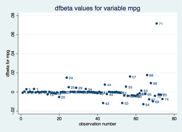
Dfbeta for grouped data

If you have panel data or a situation where each individual is represented by a group of observations (for example, conditional logit or survival models), you might be interested in influential groups. In this case, you would look at the changes on the parameters when each group is suppressed. Let’s see an example with xtlogit.

. webuse towerlondon, clear
. xtset family

. jackknife, cluster(family) idcluster(newclus) keep: xtlogit dtlm difficulty
. assert e(N_misreps)==0

The group-level pseudovalues will be saved on the first observations corresponding to each group, and there will be missing values on the rest. To compute the dfbeta value for the coefficient for difficulty, we type

. local N = e(N_clust)
. gen dfbeta_difficulty = (dtlm_b_difficulty - _b[difficulty])/(`N'-1)

We can then plot those values:

. scatter dfbeta_difficulty newclus, mlabel(family) ///
       title("dfbeta values for variable difficulty") xtitle("family")

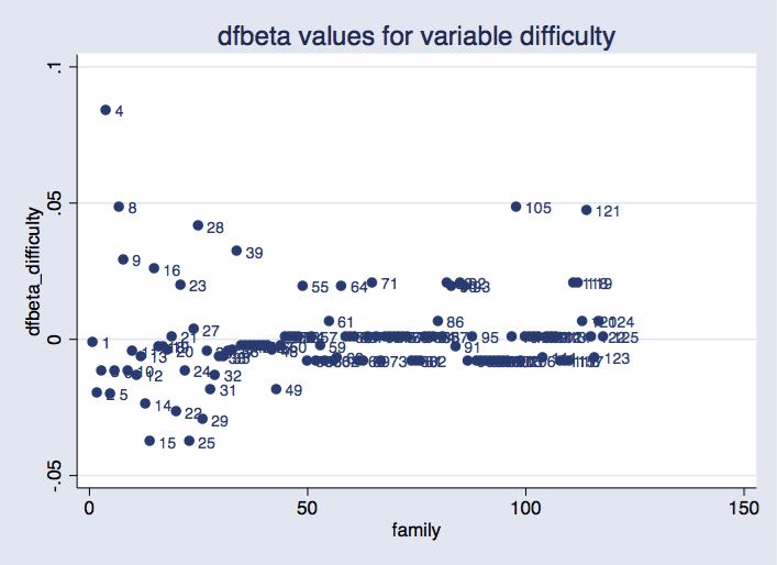
Option idcluster() for jackknife generates a new variable that assigns consecutive integers to the clusters; using this variable produces a plot where families are equally spaced on the horizontal axis.

As before, we can see that some groups are more influential than others. It would require some research to find out whether this is a problem.

Likelihood displacement

If we want a global measure of influence (that is, not tied to a particular parameter), we can compute the likelihood displacement values. We consider the likelihood displacement value as defined by Cook (1986):

\[LD_i = 2[L(\hat\theta) - L(\hat\theta_{(i)})] \]

where \(L\) is the log-likelihood function (evaluated on the full dataset), \(\hat\theta\) is the set of parameter estimates obtained from the full dataset, and \(\hat\theta_{(i)}\) is the set of the parameter estimates obtained when leaving out the \(i\)th observation. Notice that what changes is the parameter vector. The log-likelihood function is always evaluated on the whole sample; provided that \(\hat\theta\) is the set of parameters that maximizes the log likelihood, the log-likelihood displacement is always positive. Cook suggested, as a confidence region for this value, the interval \([0, \chi^2_p(\alpha))\), where \(\chi^2_p(\alpha)\) is the (\(1-\alpha\)) quantile from a chi-squared distribution with \(p\) degrees of freedom, and \(p\) is the number of parameters in \(\theta\).

To perform our assessment based on the likelihood displacement, we will need to do the following:

1. Create an \(N\times p\) matrix B, where the \(i\)th row contains the vector of parameter estimates obtained by leaving the \(i\)th observation out.
2. Create a new variable L1 such that its \(i\)th observation contains the log likelihood evaluated at the parameter estimates in the \(i\)th row of matrix B.
3. Use variable L1 to obtain the LD matrix, containing the likelihood displacement values.
4. Construct a plot for the values in LD, and add the \(\chi^2_p(\alpha)\) as a reference.

Let's do it with our probit model.

Step 1.

We first create the macro cmdline containing the command line for the model we want to use. We fit the model and save the original log likelihood in macro ll0.

With a loop, the leave-one-out parameters are saved in consecutive rows of matrix B. It is useful to have those values in a matrix, because we will then extract each row to evaluate the log likelihood at those values.

**********Step 1
sysuse auto, clear
set more off
local cmdline probit foreign weight mpg
`cmdline'
keep if e(sample)
local ll0 = e(ll)
mat b0 = e(b)
mat b = b0

local N = _N

forvalues i = 1(1)`N'{
   `cmdline' if _n !=`i'
   mat b1 = e(b)
   mat b = b \ b1
}

mat B = b[2...,1...]
mat list B

Step 2.

In each iteration of a loop, a row from B is stored as matrix b. To evaluate the log likelihood at these values, the trick is to use them as initial values and invoke the command with 0 iterations. This can be done for any command that is based on ml.

**********Step 2

gen L1 = .

forvalues i = 1(1)`N'{
    mat b = B[`i',1...]
    `cmdline', from(b) iter(0)
    local ll = e(ll)
    replace L1 = `ll' in `i'
}

Step 3.

Using variable L1 and the macro with the original log likelihood, we compute Cook's likehood displacement.

**********Step 3

gen LD = 2*(`ll0' - L1)

Step 4.

Create the plot, using as a reference the 90% quantile for the \(\chi^2\) distribution. \(p\) is the number of columns in matrix b0 (or equivalently, the number of columns in matrix B).

**********Step 4

local k = colsof(b0)
gen upper_bound = invchi2tail(`k', .1)
gen n = _n

twoway scatter LD n, mlabel(n) || line upper_bound n, ///
title("Likelihood displacement")

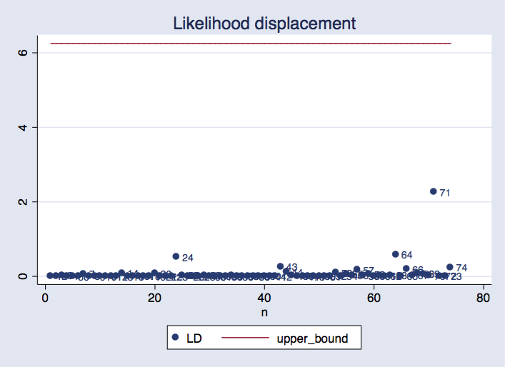
We can see that observation 71 is the most influential, and its likelihood displacement value is within the range we would normally expect.

Reference

Cook, D. 1986. Assessment of local influence. Journal of the Royal Statistical Society, Series B 48: 133–169.

I was recently talking with my friend Rebecca about simulating multilevel data, and she asked me if I would show her some examples. It occurred to me that many of you might also like to see some examples, so I decided to post them to the Stata Blog.

Introduction

We simulate data all the time at StataCorp and for a variety of reasons.

One reason is that real datasets that include the features we would like are often difficult to find. We prefer to use real datasets in the manual examples, but sometimes that isn’t feasible and so we create simulated datasets.

We also simulate data to check the coverage probabilities of new estimators in Stata. Sometimes the formulae published in books and papers contain typographical errors. Sometimes the asymptotic properties of estimators don’t hold under certain conditions. And every once in a while, we make coding mistakes. We run simulations during development to verify that a 95% confidence interval really is a 95% confidence interval.

Simulated data can also come in handy for presentations, teaching purposes, and calculating statistical power using simulations for complex study designs.

And, simulating data is just plain fun once you get the hang of it.

Some of you will recall Vince Wiggins’s blog entry from 2011 entitled “Multilevel random effects in xtmixed and sem — the long and wide of it” in which he simulated a three-level dataset. I’m going to elaborate on how Vince simulated multilevel data, and then I’ll show you some useful variations. Specifically, I’m going to talk about:

1. How to simulate single-level data
2. How to simulate two- and three-level data
3. How to simulate three-level data with covariates
4. How to simulate longitudinal data with random slopes
5. How to simulate longitudinal data with structured errors

How to simulate single-level data

Let’s begin by simulating a trivially simple, single-level dataset that has the form

\[y_i = 70 + e_i\]

We will assume that e is normally distributed with mean zero and variance \(\sigma^2\).

We’d want to simulate 500 observations, so let’s begin by clearing Stata’s memory and setting the number of observations to 500.

. clear 
. set obs 500

Next, let’s create a variable named e that contains pseudorandom normally distributed data with mean zero and standard deviation 5:

. generate e = rnormal(0,5)

The variable e is our error term, so we can create an outcome variable y by typing

. generate y = 70 + e

. list y e in 1/5

     +----------------------+
     |        y           e |
     |----------------------|
  1. | 78.83927     8.83927 |
  2. | 69.97774   -.0222647 |
  3. | 69.80065   -.1993514 |
  4. | 68.11398    -1.88602 |
  5. | 63.08952   -6.910483 |
     +----------------------+

We can fit a linear regression for the variable y to determine whether our parameter estimates are reasonably close to the parameters we specified when we simulated our dataset:

. regress y

      Source |       SS       df       MS              Number of obs =     500
-------------+------------------------------           F(  0,   499) =    0.00
       Model |           0     0           .           Prob > F      =       .
    Residual |  12188.8118   499  24.4264766           R-squared     =  0.0000
-------------+------------------------------           Adj R-squared =  0.0000
       Total |  12188.8118   499  24.4264766           Root MSE      =  4.9423

------------------------------------------------------------------------------
           y |      Coef.   Std. Err.      t    P>|t|     [95% Conf. Interval]
-------------+----------------------------------------------------------------
       _cons |   69.89768    .221027   316.24   0.000     69.46342    70.33194
------------------------------------------------------------------------------

The estimate of _cons is 69.9, which is very close to 70, and the Root MSE of 4.9 is equally close to the error’s standard deviation of 5. The parameter estimates will not be exactly equal to the underlying parameters we specified when we created the data because we introduced randomness with the rnormal() function.

This simple example is just to get us started before we work with multilevel data. For familiarity, let’s fit the same model with the mixed command that we will be using later:

. mixed y, stddev

Mixed-effects ML regression                     Number of obs      =       500

                                                Wald chi2(0)       =         .
Log likelihood = -1507.8857                     Prob > chi2        =         .

------------------------------------------------------------------------------
           y |      Coef.   Std. Err.      z    P>|z|     [95% Conf. Interval]
-------------+----------------------------------------------------------------
       _cons |   69.89768   .2208059   316.56   0.000     69.46491    70.33045
------------------------------------------------------------------------------

------------------------------------------------------------------------------
  Random-effects Parameters  |   Estimate   Std. Err.     [95% Conf. Interval]
-----------------------------+------------------------------------------------
                sd(Residual) |    4.93737   .1561334      4.640645    5.253068
------------------------------------------------------------------------------

The output is organized with the parameter estimates for the fixed part in the top table and the estimated standard deviations for the random effects in the bottom table. Just as previously, the estimate of _cons is 69.9, and the estimate of the standard deviation of the residuals is 4.9.

Okay. That really was trivial, wasn’t it? Simulating two- and three-level data is almost as easy.

How to simulate two- and three-level data

I posted a blog entry last year titled “Multilevel linear models in Stata, part 1: Components of variance“. In that posting, I showed a diagram for a residual of a three-level model.

The equation for the variance-components model I fit had the form

\[y_{ijk} = mu + u_i.. + u_{ij.} + e_{ijk}\]

This model had three residuals, whereas the one-level model we just fit above had only one.

This time, let’s start with a two-level model. Let’s simulate a two-level dataset, a model for children nested within classrooms. We’ll index classrooms by i and children by j. The model is
\[y_{ij} = mu + u_{i.} + e_{ij}\]

For this toy model, let’s assume two classrooms with two students per classroom, meaning that we want to create a four-observation dataset, where the observations are students.

To create this four-observation dataset, we start by creating a two-observation dataset, where the observations are classrooms. Because there are two classrooms, we type

. clear 
. set obs 2
. generate classroom = _n

From now on, we’ll refer to classroom as i. It’s easier to remember what variables mean if they have meaningful names.

Next, we’ll create a variable that contains each classroom’s random effect \(u_i\), which we’ll assume follows an N(0,3) distribution.

. generate u_i = rnormal(0,3)

. list

     +----------------------+
     | classr~m         u_i |
     |----------------------|
  1. |        1    .7491351 |
  2. |        2   -.0031386 |
     +----------------------+

We can now expand our data to include two children per classroom by typing

. expand 2

. list

     +----------------------+
     | classr~m         u_i |
     |----------------------|
  1. |        1    .7491351 |
  2. |        2   -.0031386 |
  3. |        1    .7491351 |
  4. |        2   -.0031386 |
     +----------------------+

Now, we can think of our observations as being students. We can create a child ID (we’ll call it child rather than j), and we can create each child’s residual \(e_{ij}\), which we will assume has an N(0,5) distribution:

. bysort classroom: generate child = _n

. generate e_ij = rnormal(0,5)

. list

     +------------------------------------------+
     | classr~m         u_i   child        e_ij |
     |------------------------------------------|
  1. |        1    .7491351       1    2.832674 |
  2. |        1    .7491351       2    1.487452 |
  3. |        2   -.0031386       1    6.598946 |
  4. |        2   -.0031386       2   -.3605778 |
     +------------------------------------------+

We now have nearly all the ingredients to calculate \(y_{ij}\):

\(y_{ij} = mu + u_{i.} + e_{ij}\)

We’ll assume mu is 70. We type

. generate y = 70 + u_i + e_ij

. list y classroom u_i child e_ij, sepby(classroom)

     +-----------------------------------------------------+
     |        y   classr~m         u_i   child        e_ij |
     |-----------------------------------------------------|
  1. | 73.58181          1    .7491351       1    2.832674 |
  2. | 72.23659          1    .7491351       2    1.487452 |
     |-----------------------------------------------------|
  3. | 76.59581          2   -.0031386       1    6.598946 |
  4. | 69.63628          2   -.0031386       2   -.3605778 |
     +-----------------------------------------------------+

Note that the random effect u_i is the same within each school, and each child has a different value for e_ij.

Our strategy was simple:

1. Start with the top level of the data hierarchy.
2. Create variables for the level ID and its random effect.
3. Expand the data by the number of observations within that level.
4. Repeat steps 2 and 3 until the bottom level is reached.

Let’s try this recipe for three-level data where children are nested within classrooms which are nested within schools. This time, I will index schools with i, classrooms with j, and children with k so that my model is

\[y_{ijk} = mu + u_{i..} + u_{ij.} + e_{ijk}\]

where

\(u_{i..}\) ~ N(0,2)
\(u_{ij.}\) ~ N(0,3)
\(u_{ijk}\) ~ N(0,5)

Let’s create data for

(level 3, i)   2 schools

(level 2, j)   2 classrooms in each school

(level 1, k)  2 students in most classrooms; 3 students in i==2 & j==2

Begin by creating the level-three data for the two schools:

. clear
. set obs 2
. generate school = _n
. generate u_i = rnormal(0,2)
. list school u_i

     +--------------------+
     | school         u_i |
     |--------------------|
  1. |      1    3.677312 |
  2. |      2   -3.193004 |
     +--------------------+

Next, we expand the data so that we have the three classrooms nested within each of the schools, and we create its random effect:

. expand 2
. bysort school: generate classroom = _n
. generate u_ij = rnormal(0,3)
. list school u_i classroom u_ij, sepby(school)

     +-------------------------------------------+
     | school         u_i   classr~m        u_ij |
     |-------------------------------------------|
  1. |      1    3.677312          1    .9811059 |
  2. |      1    3.677312          2   -3.482453 |
     |-------------------------------------------|
  3. |      2   -3.193004          1   -4.107915 |
  4. |      2   -3.193004          2   -2.450383 |
     +-------------------------------------------+

Finally, we expand the data so that we have three students in school 2′s classroom 2, and two students in all the other classrooms. Sorry for that complication, but I wanted to show you how to create unbalanced data.

In the previous examples, we’ve been typing things like expand 2, meaning double the observations. In this case, we need to do something different for school 2, classroom 2, namely,

. expand 3 if school==2 & classroom==2

and then we can just expand the rest:

. expand 2 if !(school==2 & clasroom==2)

Obviously, in a real simulation, you would probably want 16 to 25 students in each classroom. You could do something like that by typing

. expand 16+int((25-16+1)*runiform())

In any case, we will type

. expand 3 if school==2 & classroom==2

. expand 2 if !(school==2 & classroom==2)

. bysort school classroom: generate child = _n

. generate e_ijk = rnormal(0,5)

. generate y = 70 + u_i + u_ij + e_ijk

. list y school u_i classroom u_ij child e_ijk, sepby(classroom)

     +------------------------------------------------------------------------+
     |        y   school       u_i   classr~m        u_ij   child       e_ijk |
     |------------------------------------------------------------------------|
  1. | 76.72794        1  3.677312          1    .9811059       1    2.069526 |
  2. | 69.81315        1  3.677312          1    .9811059       2   -4.845268 |
     |------------------------------------------------------------------------|
  3. | 74.09565        1  3.677312          2   -3.482453       1    3.900788 |
  4. | 71.50263        1  3.677312          2   -3.482453       2    1.307775 |
     |------------------------------------------------------------------------|
  5. | 64.86206        2 -3.193004          1   -4.107915       1    2.162977 |
  6. | 61.80236        2 -3.193004          1   -4.107915       2   -.8967164 |
     |------------------------------------------------------------------------|
  7. | 66.65285        2 -3.193004          2   -2.450383       1    2.296242 |
  8. | 49.96139        2 -3.193004          2   -2.450383       2   -14.39522 |
  9. | 64.41605        2 -3.193004          2   -2.450383       3    .0594433 |
     +------------------------------------------------------------------------+

Regardless of how we generate the data, we must ensure that the school-level random effects u_i are the same within school and the classroom-level random effects u_ij are the same within classroom.

Concerning data construction, the example above we concocted to produce a dataset that would be easy to list. Let’s now create a dataset that is more reasonable:

\[y_{ijk} = mu + u_{i..} + u_{ij.} + e_{ijk}\]

where

\(u_{i..}\) ~ N(0,2)
\(u_{ij.}\) ~ N(0,3)
\(u_{ijk}\) ~ N(0,5)

Let’s create data for

(level 3, i)   6 schools

(level 2, j)   10 classrooms in each school

(level 1, k)   16-25 students

. clear
. set obs 6
. generate school = _n
. generate u_i = rnormal(0,2)
. expand 10
. bysort school: generate classroom = _n
. generate u_ij = rnormal(0,3)
. expand 16+int((25-16+1)*runiform())
. bysort school classroom: generate child = _n
. generate e_ijk = rnormal(0,5)
. generate y = 70 + u_i + u_ij + e_ijk

We can use the mixed command to fit the model with our simulated data.

. mixed y || school: || classroom: , stddev

Mixed-effects ML regression                     Number of obs      =      1217

-----------------------------------------------------------
                |   No. of       Observations per Group
 Group Variable |   Groups    Minimum    Average    Maximum
----------------+------------------------------------------
         school |        6        197      202.8        213
      classroom |       60         16       20.3         25
-----------------------------------------------------------

                                                Wald chi2(0)       =         .
Log likelihood = -3710.0673                     Prob > chi2        =         .

------------------------------------------------------------------------------
           y |      Coef.   Std. Err.      z    P>|z|     [95% Conf. Interval]
-------------+----------------------------------------------------------------
       _cons |   70.25941   .9144719    76.83   0.000     68.46707    72.05174
------------------------------------------------------------------------------

------------------------------------------------------------------------------
  Random-effects Parameters  |   Estimate   Std. Err.     [95% Conf. Interval]
-----------------------------+------------------------------------------------
school: Identity             |
                   sd(_cons) |   2.027064   .7159027      1.014487    4.050309
-----------------------------+------------------------------------------------
classroom: Identity          |
                   sd(_cons) |   2.814152   .3107647       2.26647    3.494178
-----------------------------+------------------------------------------------
                sd(Residual) |   4.828923   .1003814      4.636133     5.02973
------------------------------------------------------------------------------
LR test vs. linear regression:       chi2(2) =   379.37   Prob > chi2 = 0.0000

The parameter estimates from our simulated data match the parameters used to create the data pretty well: the estimate for _cons is 70.3, which is near 70; the estimated standard deviation for the school-level random effects is 2.02, which is near 2; the estimated standard deviation for the classroom-level random effects is 2.8, which is near 3; and the estimated standard deviation for the individual-level residuals is 4.8, which is near 5.

We’ve just done one reasonable simulation.

If we wanted to do a full simulation, we would need to do the above 100, 1,000, 10,000, or more times. We would put our code in a loop. And in that loop, we would keep track of whatever parameter interested us.

How to simulate three-level data with covariates

Usually, we’re more interested in estimating the effects of the covariates than in estimating the variance of the random effects. Covariates are typically binary (such as male/female), categorical (such as race), ordinal (such as education level), or continuous (such as age).

Let’s add some covariates to our simulated data. Our model is

\[y_{ijk} = mu + u_{i..} + u_{ij.} + e_{ijk}\]

where

\(u_{i..}\) ~ N(0,2)
\(u_{ij.}\) ~ N(0,3)
\(u_{ijk}\) ~ N(0,5)

We create data for

(level 3, i)   6 schools

(level 2, j)   10 classrooms in each school

(level 1, k)   16-25 students

Let’s add to this model

(level 3, school i)       whether the school is in an urban environment

(level 2, classroom j)  teacher’s experience (years)

(level 1, student k)    student’s mother’s education level

We can create a binary covariate called urban at the school level that equals 1 if the school is located in an urban area and equals 0 otherwise.

. clear
. set obs 6
. generate school = _n
. generate u_i = rnormal(0,2)
. generate urban = runiform()<0.50

Here we assigned schools to one of the two groups with equal probability (runiform()<0.50), but we could have assigned 70% of the schools to be urban by typing

. generate urban = runiform()<0.70

At the classroom level, we could add a continuous covariate for the teacher's years of experience. We could generate this variable by using any of Stata's random-number functions (see help random_number_functions. In the example below, I've generated teacher's years of experience with a uniform distribution ranging from 5-20 years.

. expand 10
. bysort school: generate classroom = _n
. generate u_ij = rnormal(0,3)
. bysort school: generate teach_exp = 5+int((20-5+1)*runiform())

When we summarize our data, we see that teaching experience ranges from 6-20 years with an average of 13 years.

. summarize teach_exp

    Variable |       Obs        Mean    Std. Dev.       Min        Max
-------------+--------------------------------------------------------
   teach_exp |        60    13.21667    4.075939          6         20

At the child level, we could add a categorical/ordinal covariate for mother's highest level of education completed. After we expand the data and create the child ID and error variables, we can generate a uniformly distributed random variable, temprand, on the interval [0,1].

. expand 16+int((25-16+1)*runiform())
. bysort school classroom: generate child = _n
. generate e_ijk = rnormal(0,5)
. generate temprand = runiform()

We can assign children to different groups by using the egen command with cutpoints. In the example below, children whose value of temprand is in the interval [0,0.5) will be assigned to mother_educ==0, children whose value of temprand is in the interval [0.5,0.9) will be assigned to mother_educ==1, and children whose value of temprand is in the interval [0.9,1) will be assigned to mother_educ==2.

. egen mother_educ = cut(temprand), at(0,0.5, 0.9, 1) icodes
. label define mother_educ 0 "HighSchool" 1 "College" 2 ">College"
. label values mother_educ mother_educ

The resulting frequencies of each category are very close to the frequencies we specified in our egen command.

. tabulate mother_educ, generate(meduc)

mother_educ |      Freq.     Percent        Cum.
------------+-----------------------------------
 HighSchool |        602       50.17       50.17
    College |        476       39.67       89.83
   >College |        122       10.17      100.00
------------+-----------------------------------
      Total |      1,200      100.00

We used the option generate(meduc) in the tabulate command above to create indicator variables for each category of mother_educ. This will allow us to specify an effect size for each category when we create our outcome variable.

. summarize meduc*

    Variable |       Obs        Mean    Std. Dev.       Min        Max
-------------+--------------------------------------------------------
      meduc1 |      1200    .5016667    .5002057          0          1
      meduc2 |      1200    .3966667    .4894097          0          1
      meduc3 |      1200    .1016667    .3023355          0          1

Now, we can create an outcome variable called score by adding all our fixed and random effects together. We can specify an effect size (regression coefficient) for each fixed effect in our model.

. generate score = 70
        + (-2)*urban
        + 1.5*teach_exp
        + 0*meduc1
        + 2*meduc2
        + 5*meduc3
        + u_i + u_ij + e_ijk

I have specified that the grand mean is 70, urban schools will have scores 2 points lower than nonurban schools, and each year of teacher's experience will add 1.5 points to the students score.

Mothers whose highest level of education was high school (meduc1==1) will serve as the referent category for mother_educ(mother_educ==0). The scores of children whose mother completed college (meduc2==1 and mother_educ==1) will be 2 points higher than the children in the referent group. And the scores of children whose mother completed more than college (meduc3==1 and mother_educ==2) will be 5 points higher than the children in the referent group. Now, we can use the mixed command to fit a model to our simulated data. We used the indicator variables meduc1-meduc3 to create the data, but we will use the factor variable i.mother_educ to fit the model.

. mixed score urban teach_exp i.mother_educ  || school: ||
                                             classroom: , stddev baselevel

Mixed-effects ML regression                     Number of obs      =      1259

-----------------------------------------------------------
                |   No. of       Observations per Group
 Group Variable |   Groups    Minimum    Average    Maximum
----------------+------------------------------------------
         school |        6        200      209.8        217
      classroom |       60         16       21.0         25
-----------------------------------------------------------

                                                Wald chi2(4)       =    387.64
Log likelihood = -3870.5395                     Prob > chi2        =    0.0000

------------------------------------------------------------------------------
       score |      Coef.   Std. Err.      z    P>|z|     [95% Conf. Interval]
-------------+----------------------------------------------------------------
       urban |  -2.606451    2.07896    -1.25   0.210    -6.681138    1.468237
   teach_exp |   1.584759    .096492    16.42   0.000     1.395638     1.77388
             |
 mother_educ |
 HighSchool  |          0  (base)
    College  |   2.215281   .3007208     7.37   0.000     1.625879    2.804683
   >College  |   5.065907   .5237817     9.67   0.000     4.039314      6.0925
             |
       _cons |   68.95018   2.060273    33.47   0.000     64.91212    72.98824
------------------------------------------------------------------------------

------------------------------------------------------------------------------
  Random-effects Parameters  |   Estimate   Std. Err.     [95% Conf. Interval]
-----------------------------+------------------------------------------------
school: Identity             |
                   sd(_cons) |   2.168154   .7713944      1.079559    4.354457
-----------------------------+------------------------------------------------
classroom: Identity          |
                   sd(_cons) |    3.06871   .3320171      2.482336    3.793596
-----------------------------+------------------------------------------------
                sd(Residual) |   4.947779   .1010263      4.753681    5.149802
------------------------------------------------------------------------------
LR test vs. linear regression:       chi2(2) =   441.25   Prob > chi2 = 0.0000

“Close” is in the eye of the beholder, but to my eyes, the parameter estimates look remarkably close to the parameters that were used to simulate the data. The parameter estimates for the fixed part of the model are -2.6 for urban (parameter = -2), 1.6 for teach_exp (parameter = 1.5), 2.2 for the College category of mother_educ (parameter = 2), 5.1 for the >College category of mother_educ (parameter = 5), and 69.0 for the intercept (parameter = 70). The estimated standard deviations for the random effects are also very close to the simulation parameters. The estimated standard deviation is 2.2 (parameter = 2) at the school level, 3.1 (parameter = 3) at the classroom level, and 4.9 (parameter = 5) at the child level.

Some of you may disagree that the parameter estimates are close. My reply is that it doesn’t matter unless you’re simulating a single dataset for demonstration purposes. If you are, simply simulate more datasets until you get one that looks close enough for you. If you are simulating data to check coverage probabilities or to estimate statistical power, you will be averaging over thousands of simulated datasets and the results of any one of those datasets won’t matter.

How to simulate longitudinal data with random slopes

Longitudinal data are often conceptualized as multilevel data where the repeated observations are nested within individuals. The main difference between ordinary multilevel models and multilevel models for longitudinal data is the inclusion of a random slope. If you are not familiar with random slopes, you can learn more about them in a blog entry I wrote last year (Multilevel linear models in Stata, part 2: Longitudinal data).

Simulating longitudinal data with a random slope is much like simulating two-level data, with a couple of modifications. First, the bottom level will be observations within person. Second, there will be an interaction between time (age) and a person-level random effect. So we will generate data for the following model:

\[weight_{ij} = mu + age_{ij} + u_{0i.} + age*u_{1i.} + e_{ij}\]

where

\(u_{0i.}\) ~ N(0,3)   \(u_{1i.}\) ~ N(0,1)   \(e_{ij}\) ~ N(0,2)

Let’s begin by simulating longitudinal data for 300 people.

. clear
. set obs 300
. gen person = _n

For longitudinal data, we must create two person-level random effects: the variable u_0i is analogous to the random effect we created earlier, and the variable u_1i is the random effect for the slope over time.

. generate u_0i = rnormal(0,3)
. generate u_1i = rnormal(0,1)

Let’s expand the data so that there are five observations nested within each person. Rather than create an observation-level identification number, let’s create a variable for age that ranges from 12 to 16 years,

. expand 5
. bysort person: generate age = _n + 11

and create an observation-level error term from an N(0,2) distribution:

. generate e_ij = rnormal(0,2)

. list person u_0i u_1i age e_ij if person==1

      +-------------------------------------------------+
      | person       u_0i        u_1i   age        e_ij |
      |-------------------------------------------------|
   1. |      1   .9338312   -.3097848    12    1.172153 |
   2. |      1   .9338312   -.3097848    13    2.935366 |
   3. |      1   .9338312   -.3097848    14   -2.306981 |
   4. |      1   .9338312   -.3097848    15   -2.148335 |
   5. |      1   .9338312   -.3097848    16   -.4276625 |
      +-------------------------------------------------+

The person-level random effects u_0i and u_1i are the same at all ages, and the observation-level random effects e_ij are different at each age. Now we’re ready to generate an outcome variable called weight, measured in kilograms, based on the following model:

\[weight_{ij} = 3 + 3.6*age_{ij} + u_{0i} + age*u_{1i} + e_{ij}\]

. generate weight = 3 + 3.6*age + u_0i + age*u_1i + e_ij

The random effect u_1i is multiplied by age, which is why it is called a random slope. We could rewrite the model as

\[weight_{ij} = 3 + age_{ij}*(3.6 + u_{1i}) + u_{01} + e_{ij}\]

Note that for each year of age, a person’s weight will increase by 3.6 kilograms plus some random amount specified by u_1j. In other words,the slope for age will be slightly different for each person.

We can use the mixed command to fit a model to our data:

. mixed weight age || person: age , stddev

Mixed-effects ML regression                     Number of obs      =      1500
Group variable: person                          Number of groups   =       300

                                                Obs per group: min =         5
                                                               avg =       5.0
                                                               max =         5


                                                Wald chi2(1)       =   3035.03
Log likelihood = -3966.3842                     Prob > chi2        =    0.0000

------------------------------------------------------------------------------
      weight |      Coef.   Std. Err.      z    P>|z|     [95% Conf. Interval]
-------------+----------------------------------------------------------------
         age |   3.708161   .0673096    55.09   0.000     3.576237    3.840085
       _cons |   2.147311   .5272368     4.07   0.000     1.113946    3.180676
------------------------------------------------------------------------------

------------------------------------------------------------------------------
  Random-effects Parameters  |   Estimate   Std. Err.     [95% Conf. Interval]
-----------------------------+------------------------------------------------
person: Independent          |
                     sd(age) |   .9979648   .0444139      .9146037    1.088924
                   sd(_cons) |    3.38705   .8425298      2.080103    5.515161
-----------------------------+------------------------------------------------
                sd(Residual) |   1.905885   .0422249      1.824897    1.990468
------------------------------------------------------------------------------
LR test vs. linear regression:       chi2(2) =  4366.32   Prob > chi2 = 0.0000

The estimate for the intercept _cons = 2.1 is not very close to the original parameter value of 3, but the estimate of 3.7 for age is very close (parameter = 3.6). The standard deviations of the random effects are also very close to the parameters used to simulate the data. The estimate for the person level _cons is 2.1 (parameter = 2), the person-level slope is 0.997 (parameter = 1), and the observation-level residual is 1.9 (parameter = 2).

How to simulate longitudinal data with structured errors

Longitudinal data often have an autoregressive pattern to their errors because of the sequential collection of the observations. Measurements taken closer together in time will be more similar than measurements taken further apart in time. There are many patterns that can be used to descibe the correlation among the errors, including autoregressive, moving average, banded, exponential, Toeplitz, and others (see help mixed##rspec).

Let’s simulate a dataset where the errors have a Toeplitz structure, which I will define below.

We begin by creating a sample with 500 people with a person-level random effect having an N(0,2) distribution.

. clear
. set obs 500
. gen person = _n
. generate u_i = rnormal(0,2)

Next, we can use the drawnorm command to create error variables with a Toeplitz pattern.

A Toeplitz 1 correlation matrix has the following structure:

. matrix V = ( 1.0, 0.5, 0.0, 0.0, 0.0  \     ///
               0.5, 1.0, 0.5, 0.0, 0.0  \     ///
               0.0, 0.5, 1.0, 0.5, 0.0  \     ///
               0.0, 0.0, 0.5, 1.0, 0.5  \     ///
               0.0, 0.0, 0.0, 0.5, 1.0 )

. matrix list V

symmetric V[5,5]
    c1  c2  c3  c4  c5
r1   1
r2  .5   1
r3   0  .5   1
r4   0   0  .5   1
r5   0   0   0  .5   1

The correlation matrix has 1s on the main diagonal, and each pair of contiguous observations will have a correlation of 0.5. Observations more than 1 unit of time away from each other are assumed to be uncorrelated.

We must also define a matrix of means to use the drawnorm command.

. matrix M = (0 \ 0 \ 0 \ 0 \ 0)

. matrix list M

M[5,1]
    c1
r1   0
r2   0
r3   0
r4   0
r5   0

Now, we’re ready to use the drawnorm command to create five error variables that have a Toeplitz 1 structure.

. drawnorm e1 e2 e3 e4 e5, means(M) cov(V)

. list in 1/2

     +---------------------------------------------------------------------------+
     | person        u_i         e1         e2        e3          e4          e5 |
     |---------------------------------------------------------------------------|
  1. |      1   5.303562  -1.288265  -1.201399   .353249    .0495944   -1.472762 |
  2. |      2  -.0133588   .6949759    2.82179  .7195075   -1.032395    .1995016 |
     +---------------------------------------------------------------------------+

Let’s estimate the correlation matrix for our simulated data to verify that our simulation worked as we expected.

. correlate e1-e5
(obs=300)

             |       e1       e2       e3       e4       e5
-------------+---------------------------------------------
          e1 |   1.0000
          e2 |   0.5542   1.0000
          e3 |  -0.0149   0.4791   1.0000
          e4 |  -0.0508  -0.0364   0.5107   1.0000
          e5 |   0.0022  -0.0615   0.0248   0.4857   1.0000

The correlations are 1 along the main diagonal, near 0.5 for the contiguous observations, and near 0 otherwise.

Our data are currently in wide format, and we need them in long format to use the mixed command. We can use the reshape command to convert our data from wide to long format. If you are not familiar with the reshape command, you can learn more about it by typing help reshape.

. reshape long e, i(person) j(time)
(note: j = 1 2 3 4 5)

Data                               wide   ->   long
-----------------------------------------------------------------------------
Number of obs.                      300   ->    1500
Number of variables                   7   ->       4
j variable (5 values)                     ->   time
xij variables:
                           e1 e2 ... e5   ->   e
-----------------------------------------------------------------------------

Now, we are ready to create our age variable and the outcome variable weight.

. bysort person: generate age = _n + 11
. generate weight = 3 + 3.6*age + u_i + e

. list weight person u_i time age e if person==1

      +-------------------------------------------------------+
      |   weight   person        u_i   time   age           e |
      |-------------------------------------------------------|
   1. |  50.2153        1   5.303562      1    12   -1.288265 |
   2. | 53.90216        1   5.303562      2    13   -1.201399 |
   3. | 59.05681        1   5.303562      3    14     .353249 |
   4. | 62.35316        1   5.303562      4    15    .0495944 |
   5. |  64.4308        1   5.303562      5    16   -1.472762 |
      +-------------------------------------------------------+

We can use the mixed command to fit a model to our simulated data.

. mixed weight age || person:, residual(toeplitz 1, t(time)) , stddev

Mixed-effects ML regression                     Number of obs      =      1500
Group variable: person                          Number of groups   =       300

                                                Obs per group: min =         5
                                                               avg =       5.0
                                                               max =         5

                                                Wald chi2(1)       =  33797.58
Log likelihood = -2323.9389                     Prob > chi2        =    0.0000

------------------------------------------------------------------------------
      weight |      Coef.   Std. Err.      z    P>|z|     [95% Conf. Interval]
-------------+----------------------------------------------------------------
         age |   3.576738   .0194556   183.84   0.000     3.538606     3.61487
       _cons |   3.119974   .3244898     9.62   0.000     2.483985    3.755962
------------------------------------------------------------------------------

------------------------------------------------------------------------------
  Random-effects Parameters  |   Estimate   Std. Err.     [95% Conf. Interval]
-----------------------------+------------------------------------------------
person: Identity             |
                   sd(_cons) |   3.004718   .1268162      2.766166    3.263843
-----------------------------+------------------------------------------------
Residual: Toeplitz(1)        |
                        rho1 |   .4977523   .0078807      .4821492    .5130398
                       sd(e) |   .9531284   .0230028      .9090933    .9992964
------------------------------------------------------------------------------
LR test vs. linear regression:       chi2(2) =  3063.87   Prob > chi2 = 0.0000

Again, our parameter estimates match the parameters that were used to simulate the data very closely.

The parameter estimate is 3.6 for age (parameter = 3.6) and 3.1 for _cons (parameter = 3). The estimated standard deviations of the person-level random effect is 3.0 (parameter = 3). The estimated standard deviation for the errors is 0.95 (parameter = 1), and the estimated correlation for the Toeplitz structure is 0.5 (parameter = 0.5).

Conclusion

I hope I’ve convinced you that simulating multilevel/longitudinal data is easy and useful. The next time you find yourself teaching a class or giving a talk that requires multilevel examples, try simulating the data. And if you need to calculate statistical power for a multilevel or longitudinal model, consider simulations.

gsem is a very flexible command that allows us to fit very sophisticated models. However, it is also useful in situations that involve simple models.

For example, when we want to compare parameters among two or more models, we usually use suest, which combines the estimation results under one parameter vector and creates a simultaneous covariance matrix of the robust type. This covariance estimate is described in the Methods and formulas of [R] suest as the robust variance from a “stacked model”. Actually, gsem can estimate these kinds of “stacked models”, even if the estimation samples are not the same and eventually overlap. By using the option vce(robust), we can replicate the results from suest if the models are available for gsem. In addition, gsem allows us to combine results from some estimation commands that are not supported by suest, like models including random effects.

Example: Comparing parameters from two models

Let’s consider the childweight dataset, described in [ME] mixed. Consider the following models, where weights of boys and girls are modeled using the age and the age-squared:

. webuse childweight, clear
(Weight data on Asian children)

. regress  weight age c.age#c.age if girl == 0, noheader
------------------------------------------------------------------------------
      weight |      Coef.   Std. Err.      t    P>|t|     [95% Conf. Interval]
-------------+----------------------------------------------------------------
         age |   7.985022   .6343855    12.59   0.000     6.725942    9.244101
             |
 c.age#c.age |   -1.74346   .2374504    -7.34   0.000    -2.214733   -1.272187
             |
       _cons |   3.684363   .3217223    11.45   0.000     3.045833    4.322893
------------------------------------------------------------------------------

. regress  weight age c.age#c.age if girl == 1, noheader
------------------------------------------------------------------------------
      weight |      Coef.   Std. Err.      t    P>|t|     [95% Conf. Interval]
-------------+----------------------------------------------------------------
         age |   7.008066   .5164687    13.57   0.000     5.982746    8.033386
             |
 c.age#c.age |  -1.450582   .1930318    -7.51   0.000    -1.833798   -1.067365
             |
       _cons |   3.480933   .2616616    13.30   0.000     2.961469    4.000397
------------------------------------------------------------------------------

To test whether birthweights are the same for the two groups, we need to test whether the intercepts in the two regressions are the same. Using suest, we would proceed as follows:

. quietly regress weight age c.age#c.age if girl == 0, noheader

. estimates store boys

. quietly regress weight age c.age#c.age if girl == 1, noheader

. estimates store girls

. suest boys girls

Simultaneous results for boys, girls

                                                  Number of obs   =        198

------------------------------------------------------------------------------
             |               Robust
             |      Coef.   Std. Err.      z    P>|z|     [95% Conf. Interval]
-------------+----------------------------------------------------------------
boys_mean    |
         age |   7.985022   .4678417    17.07   0.000     7.068069    8.901975
             |
 c.age#c.age |   -1.74346   .2034352    -8.57   0.000    -2.142186   -1.344734
             |
       _cons |   3.684363   .1719028    21.43   0.000      3.34744    4.021286
-------------+----------------------------------------------------------------
boys_lnvar   |
       _cons |   .4770289   .1870822     2.55   0.011     .1103546    .8437032
-------------+----------------------------------------------------------------
girls_mean   |
         age |   7.008066   .4166916    16.82   0.000     6.191365    7.824766
             |
 c.age#c.age |  -1.450582   .1695722    -8.55   0.000    -1.782937   -1.118226
             |
       _cons |   3.480933   .1556014    22.37   0.000      3.17596    3.785906
-------------+----------------------------------------------------------------
girls_lnvar  |
       _cons |   .0097127   .1351769     0.07   0.943    -.2552292    .2746545
------------------------------------------------------------------------------

Invoking an estimation command with the option coeflegend will give us a legend we can use to refer to the parameters when we use postestimation commands like test.

. suest, coeflegend

Simultaneous results for boys, girls

                                                  Number of obs   =        198

------------------------------------------------------------------------------
             |      Coef.  Legend
-------------+----------------------------------------------------------------
boys_mean    |
         age |   7.985022  _b[boys_mean:age]
             |
 c.age#c.age |   -1.74346  _b[boys_mean:c.age#c.age]
             |
       _cons |   3.684363  _b[boys_mean:_cons]
-------------+----------------------------------------------------------------
boys_lnvar   |
       _cons |   .4770289  _b[boys_lnvar:_cons]
-------------+----------------------------------------------------------------
girls_mean   |
         age |   7.008066  _b[girls_mean:age]
             |
 c.age#c.age |  -1.450582  _b[girls_mean:c.age#c.age]
             |
       _cons |   3.480933  _b[girls_mean:_cons]
-------------+----------------------------------------------------------------
girls_lnvar  |
       _cons |   .0097127  _b[girls_lnvar:_cons]
------------------------------------------------------------------------------

. test  _b[boys_mean:_cons] = _b[girls_mean:_cons]

 ( 1)  [boys_mean]_cons - [girls_mean]_cons = 0

           chi2(  1) =    0.77
         Prob > chi2 =    0.3803

We find no evidence that the intercepts are different.

Now, let’s replicate those results by using the gsem command. We generate the variable weightboy, a copy of weight for boys and missing otherwise, and the variable weightgirl, a copy of weight for girls and missing otherwise.

. quietly generate weightboy = weight if girl == 0

. quietly generate weightgirl = weight if girl == 1

. gsem (weightboy <- age c.age#c.age) (weightgirl <- age c.age#c.age), ///
>      nolog vce(robust)

Generalized structural equation model             Number of obs   =        198
Log pseudolikelihood =  -302.2308

-------------------------------------------------------------------------------
                 |              Robust
                 |      Coef.  Std. Err.     z   P>|z|     [95% Conf. Interval]
-----------------+-------------------------------------------------------------
weightboy <-     |
             age |   7.985022  .4678417   17.07  0.000     7.068069    8.901975
                 |
     c.age#c.age |   -1.74346  .2034352   -8.57  0.000    -2.142186   -1.344734
                 |
           _cons |   3.684363  .1719028   21.43  0.000      3.34744    4.021286
-----------------+-------------------------------------------------------------
weightgirl <-    |
             age |   7.008066  .4166916   16.82  0.000     6.191365    7.824766
                 |
     c.age#c.age |  -1.450582  .1695722   -8.55  0.000    -1.782937   -1.118226
                 |
           _cons |   3.480933  .1556014   22.37  0.000      3.17596    3.785906
-----------------+-------------------------------------------------------------
 var(e.weightboy)|   1.562942  .3014028                    1.071012    2.280821
var(e.weightgirl)|    .978849  .1364603                    .7448187    1.286414
-------------------------------------------------------------------------------

. gsem, coeflegend

Generalized structural equation model             Number of obs   =        198
Log pseudolikelihood =  -302.2308

-------------------------------------------------------------------------------
                 |      Coef.  Legend
-----------------+-------------------------------------------------------------
weightboy <-     |
             age |   7.985022  _b[weightboy:age]
                 |
     c.age#c.age |   -1.74346  _b[weightboy:c.age#c.age]
                 |
           _cons |   3.684363  _b[weightboy:_cons]
-----------------+-------------------------------------------------------------
weightgirl <-    |
             age |   7.008066  _b[weightgirl:age]
                 |
     c.age#c.age |  -1.450582  _b[weightgirl:c.age#c.age]
                 |
           _cons |   3.480933  _b[weightgirl:_cons]
-----------------+-------------------------------------------------------------
 var(e.weightboy)|   1.562942  _b[var(e.weightboy):_cons]
var(e.weightgirl)|    .978849  _b[var(e.weightgirl):_cons]
-------------------------------------------------------------------------------

. test  _b[weightgirl:_cons]=  _b[weightboy:_cons]

 ( 1)  - [weightboy]_cons + [weightgirl]_cons = 0

           chi2(  1) =    0.77
         Prob > chi2 =    0.3803

gsem allowed us to fit models on different subsets simultaneously. By default, the model is assumed to be a linear regression, but several links and families are available; for example, you can combine two Poisson models or a multinomial logistic model with a regular logistic model. See [SEM] sem and gsem for details.

Here, I use the vce(robust) option to replicate the results for suest. However, when estimation samples don’t overlap, results from both estimations are assumed to be independent, and thus the option vce(robust) is not needed. When performing the estimation without the vce(robust) option, the joint covariance matrix will contain two blocks with the covariances from the original models and 0s outside those blocks.

An example with random effects

The childweight dataset contains repeated measures, and it is, in the documentation, analyzed used the mixed command, which allows us to account for the intra-individual correlation via random effects.

Now, let’s use the techniques described above to combine results from two random-effects models. Here are the two separate models:

. mixed weight age c.age#c.age if girl == 0 || id:, nolog

Mixed-effects ML regression                     Number of obs      =       100
Group variable: id                              Number of groups   =        34

                                                Obs per group: min =         1
                                                               avg =       2.9
                                                               max =         5


                                                Wald chi2(2)       =   1070.28
Log likelihood = -149.05479                     Prob > chi2        =    0.0000

------------------------------------------------------------------------------
      weight |      Coef.   Std. Err.      z    P>|z|     [95% Conf. Interval]
-------------+----------------------------------------------------------------
         age |   8.328882   .4601093    18.10   0.000     7.427084    9.230679
             |
 c.age#c.age |  -1.859798   .1722784   -10.80   0.000    -2.197458   -1.522139
             |
       _cons |   3.525929   .2723617    12.95   0.000      2.99211    4.059749
------------------------------------------------------------------------------

------------------------------------------------------------------------------
  Random-effects Parameters  |   Estimate   Std. Err.     [95% Conf. Interval]
-----------------------------+------------------------------------------------
id: Identity                 |
                  var(_cons) |   .7607779   .2439115      .4058409    1.426133
-----------------------------+------------------------------------------------
               var(Residual) |   .7225673   .1236759      .5166365    1.010582
------------------------------------------------------------------------------
LR test vs. linear regression: chibar2(01) =    30.34 Prob >= chibar2 = 0.0000

. mixed weight age c.age#c.age if girl == 1 || id:, nolog

Mixed-effects ML regression                     Number of obs      =        98
Group variable: id                              Number of groups   =        34

                                                Obs per group: min =         1
                                                               avg =       2.9
                                                               max =         5


                                                Wald chi2(2)       =   2141.72
Log likelihood =  -114.3008                     Prob > chi2        =    0.0000

------------------------------------------------------------------------------
      weight |      Coef.   Std. Err.      z    P>|z|     [95% Conf. Interval]
-------------+----------------------------------------------------------------
         age |   7.273082   .3167266    22.96   0.000     6.652309    7.893854
             |
 c.age#c.age |  -1.538309    .118958   -12.93   0.000    -1.771462   -1.305156
             |
       _cons |   3.354834   .2111793    15.89   0.000      2.94093    3.768738
------------------------------------------------------------------------------

------------------------------------------------------------------------------
  Random-effects Parameters  |   Estimate   Std. Err.     [95% Conf. Interval]
-----------------------------+------------------------------------------------
id: Identity                 |
                  var(_cons) |   .6925554   .1967582       .396848    1.208606
-----------------------------+------------------------------------------------
               var(Residual) |   .3034231   .0535359      .2147152    .4287799
------------------------------------------------------------------------------
LR test vs. linear regression: chibar2(01) =    47.42 Prob >= chibar2 = 0.0000

Random effects can be included in a gsem model by incorporating latent variables at the group level; these are the latent variables M1[id] and M2[id] below. By default, gsem will try to estimate a covariance when it sees two latent variables at the same level. This can be easily solved by restricting this covariance term to 0. Option vce(robust) should be used whenever we want to produce the mechanism used by suest.

. gsem (weightboy <- age c.age#c.age M1[id])   ///
>      (weightgirl <- age c.age#c.age M2[id]), ///
>      cov(M1[id]*M2[id]@0) vce(robust) nolog

Generalized structural equation model             Number of obs   =        198
Log pseudolikelihood = -263.35559

 ( 1)  [weightboy]M1[id] = 1
 ( 2)  [weightgirl]M2[id] = 1
                                      (Std. Err. adjusted for clustering on id)
-------------------------------------------------------------------------------
                 |              Robust
                 |      Coef.  Std. Err.     z   P>|z|     [95% Conf. Interval]
-----------------+-------------------------------------------------------------
weightboy <-     |
             age |   8.328882  .4211157   19.78  0.000      7.50351    9.154253
                 |
     c.age#c.age |  -1.859798  .1591742  -11.68  0.000    -2.171774   -1.547823
                 |
          M1[id] |          1 (constrained)
                 |
           _cons |   3.525929  .1526964   23.09  0.000      3.22665    3.825209
-----------------+-------------------------------------------------------------
weightgirl <-    |
             age |   7.273082  .3067378   23.71  0.000     6.671887    7.874277
                 |
     c.age#c.age |  -1.538309   .120155  -12.80  0.000    -1.773808    -1.30281
                 |
          M2[id] |          1 (constrained)
                 |
           _cons |   3.354834  .1482248   22.63  0.000     3.064319     3.64535
-----------------+-------------------------------------------------------------
      var(M1[id])|   .7607774  .2255575                     .4254915    1.360268
      var(M2[id])|   .6925553  .1850283                    .4102429    1.169144
-----------------+-------------------------------------------------------------
 var(e.weightboy)|   .7225674  .1645983                     .4623572    1.129221
var(e.weightgirl)|   .3034231  .0667975                    .1970877    .4671298
-------------------------------------------------------------------------------

Above, we have the joint output from the two models, which would allow us to perform tests among parameters in both models. Notice that option vce(robust) implies that standard errors will be clustered on the groups determined by id.

gsem, when called with the vce(robust) option, will complain if there are inconsistencies among the groups in the models (for example, if the random effects in both models were crossed).

Checking that you are fitting the same model

In the previous model, gsem‘s default covariance structure included a term that wasn’t in the original two models, so we needed to include an additional restriction. This can be easy to spot in a simple model, but if you don’t want to rely just on a visual inspection, you can write a small loop to make sure that all the estimates in the joint model are actually also in the original models.

Let’s see an example with random effects, this time with overlapping data.

. *fit first model and save the estimates
. gsem (weightboy <- age c.age#c.age M1[id]), nolog

Generalized structural equation model             Number of obs   =        100
Log likelihood = -149.05479

 ( 1)  [weightboy]M1[id] = 1
-------------------------------------------------------------------------------
                |      Coef.  Std. Err.     z    P>|z|     [95% Conf. Interval]
----------------+--------------------------------------------------------------
weightboy <-    |
            age |   8.328882  .4609841   18.07   0.000     7.425369    9.232394
                |
    c.age#c.age |  -1.859798  .1725233  -10.78   0.000    -2.197938   -1.521659
                |
         M1[id] |          1 (constrained)
                |
          _cons |   3.525929  .2726322   12.93   0.000      2.99158    4.060279
----------------+--------------------------------------------------------------
     var(M1[id])|   .7607774  .2439114                     .4058407    1.426132
----------------+--------------------------------------------------------------
var(e.weightboy)|   .7225674  .1236759                     .5166366    1.010582
-------------------------------------------------------------------------------

. mat b1 = e(b)

. *fit second model and save the estimates
. gsem (weight <- age M2[id]), nolog

Generalized structural equation model             Number of obs   =        198
Log likelihood = -348.32402

 ( 1)  [weight]M2[id] = 1
------------------------------------------------------------------------------
             |      Coef.   Std. Err.      z    P>|z|     [95% Conf. Interval]
-------------+----------------------------------------------------------------
weight <-    |
         age |   3.389281   .1152211    29.42   0.000     3.163452    3.615111
             |
      M2[id] |          1  (constrained)
             |
       _cons |   5.156913   .1803059    28.60   0.000      4.80352    5.510306
-------------+----------------------------------------------------------------
  var(M2[id])|   .6076662   .2040674                      .3146395    1.173591
-------------+----------------------------------------------------------------
var(e.weight)|   1.524052   .1866496                      1.198819    1.937518
------------------------------------------------------------------------------

. mat b2 = e(b)

. *stack estimates from first and second models
. mat stacked = b1, b2

. *estimate joint model and save results
. gsem (weightboy <- age c.age#c.age M1[id]) ///
>      (weight <- age M2[id]), cov(M1[id]*M2[id]@0) vce(robust) nolog

Generalized structural equation model             Number of obs   =        198
Log pseudolikelihood = -497.37881

 ( 1)  [weightboy]M1[id] = 1
 ( 2)  [weight]M2[id] = 1
                                      (Std. Err. adjusted for clustering on id)
-------------------------------------------------------------------------------
                |              Robust
                |      Coef.  Std. Err.     z    P>|z|     [95% Conf. Interval]
----------------+--------------------------------------------------------------
weightboy <-    |
            age |   8.328882  .4211157   19.78   0.000      7.50351    9.154253
                |
    c.age#c.age |  -1.859798  .1591742  -11.68   0.000    -2.171774   -1.547823
                |
         M1[id] |          1 (constrained)
                |
          _cons |   3.525929  .1526964   23.09   0.000      3.22665    3.825209
----------------+--------------------------------------------------------------
weight <-       |
            age |   3.389281  .1157835   29.27   0.000      3.16235    3.616213
                |
         M2[id] |          1 (constrained)
                |
          _cons |   5.156913  .1345701   38.32   0.000      4.89316    5.420665
----------------+--------------------------------------------------------------
     var(M1[id])|   .7607774  .2255575                     .4254915    1.360268
     var(M2[id])|   .6076662     .1974                     .3214791    1.148623
----------------+--------------------------------------------------------------
var(e.weightboy)|   .7225674  .1645983                     .4623572    1.129221
   var(e.weight)|   1.524052  .1705637                     1.223877    1.897849
-------------------------------------------------------------------------------

. mat b = e(b)

. *verify that estimates from the joint model are the same as
. *from models 1 and 2
. local stripes : colfullnames(b)

. foreach l of local stripes{
  2.    matrix  r1 =  b[1,"`l'"]
  3.    matrix r2 = stacked[1,"`l'"]
  4.    assert reldif(el(r1,1,1), el(r2,1,1))<1e-5
  5. }

The loop above verifies that all the labels in the second model correspond to estimates in the first and that the estimates are actually the same. If you omit the restriction for the variance in the joint model, the assert command will produce an error.

Technical note

As documented in [U] 20.21.2 Correlated errors: Cluster-robust standard errors, the formula for the robust estimator of the variance is

\[
V_{robust} = \hat V(\sum_{j=1}^N u'_ju_j) \hat V
\]

where \(N\) is the number of observations, \(\hat V\) is the conventional estimator of the variance, and for each observation \(j\), \(u_j\) is a row vector (with as many columns as parameters), which represents the contribution of this observation to the gradient. (If we stack the rows \(u_j\), the columns of this matrix are the scores.)

When we apply suest, the matrix \(\hat V\) is constructed as the stacked block-diagonal conventional variance estimates from the original submodels; this is the variance you will see if you apply gsem to the joint model without the vce(robust) option. The \(u_j\) values used by suest are now the values from both estimations, so we have as many \(u_j\) values as the sum of observations in the two original models and each row contains as many columns as the total number of parameters in both models. This is the exact operation that gsem, vce(robust) does.

When random effects are present, standard errors will be clustered on groups. Instead of observation-level contributions to the gradient, we would use cluster-level contributions. This means that observations in the two models would need to be clustered in a consistent manner; observations that are common to the two estimations would need to be in the same cluster in the two estimations.

Two-step estimation problems can be solved using the gmm command.

When a two-step estimator produces consistent point estimates but inconsistent standard errors, it is known as the two-step-estimation problem. For instance, inverse-probability weighted (IPW) estimators are a weighted average in which the weights are estimated in the first step. Two-step estimators use first-step estimates to estimate the parameters of interest in a second step. The two-step-estimation problem arises because the second step ignores the estimation error in the first step.

One solution is to convert the two-step estimator into a one-step estimator. My favorite way to do this conversion is to stack the equations solved by each of the two estimators and solve them jointly. This one-step approach produces consistent point estimates and consistent standard errors. There is no two-step problem because all the computations are performed jointly. Newey (1984) derives and justifies this approach.

I’m going to illustrate this approach with the IPW example, but it can be used with any two-step problem as long as each step is continuous.

IPW estimators are frequently used to estimate the mean that would be observed if everyone in a population received a specified treatment, a quantity known as a potential-outcome mean (POM). A difference of POMs is called the average treatment effect (ATE). Aside from all that, it is the mechanics of the two-step IPW estimator that interest me here. IPW estimators are weighted averages of the outcome, and the weights are estimated in a first step. The weights used in the second step are the inverse of the estimated probability of treatment.

Let’s imagine we are analyzing an extract of the birthweight data used by Cattaneo (2010). In this dataset, bweight is the baby’s weight at birth, mbsmoke is 1 if the mother smoked while pregnant (and 0 otherwise), mmarried is 1 if the mother is married, and prenatal1 is 1 if the mother had a prenatal visit in the first trimester.

Let’s imagine we want to estimate the mean when all pregnant women smoked, which is to say, the POM for smoking. If we were doing substantive research, we would also estimate the POM when no pregnant women smoked. The difference between these estimated POMs would then estimate the ATE of smoking.

In the IPW estimator, we begin by estimating the probability weights for smoking. We fit a probit model of mbsmoke as a function of mmarried and prenatal1.

. use cattaneo2
(Excerpt from Cattaneo (2010) Journal of Econometrics 155: 138-154)

. probit mbsmoke mmarried prenatal1, vce(robust)

Iteration 0:   log pseudolikelihood = -2230.7484
Iteration 1:   log pseudolikelihood = -2102.6994
Iteration 2:   log pseudolikelihood = -2102.1437
Iteration 3:   log pseudolikelihood = -2102.1436

Probit regression                                 Number of obs   =       4642
                                                  Wald chi2(2)    =     259.42
                                                  Prob > chi2     =     0.0000
Log pseudolikelihood = -2102.1436                 Pseudo R2       =     0.0577

------------------------------------------------------------------------------
             |               Robust
     mbsmoke |      Coef.   Std. Err.      z    P>|z|     [95% Conf. Interval]
-------------+----------------------------------------------------------------
    mmarried |  -.6365472   .0478037   -13.32   0.000    -.7302407   -.5428537
   prenatal1 |  -.2144569   .0547583    -3.92   0.000    -.3217811   -.1071327
       _cons |  -.3226297   .0471906    -6.84   0.000    -.4151215   -.2301379
------------------------------------------------------------------------------

The results indicate that both mmarried and prenatal1 significantly predict whether the mother smoked while pregnant.

We want to calculate the inverse probabilities. We begin by getting the probabilities:

. predict double pr, pr

Now, we can obtain the inverse probabilities by typing

. generate double ipw = (mbsmoke==1)/pr

We can now perform the second step: calculate the mean for smokers by using the IPWs.

. mean bweight [pw=ipw]

Mean estimation                     Number of obs    =     864

--------------------------------------------------------------
             |       Mean   Std. Err.     [95% Conf. Interval]
-------------+------------------------------------------------
     bweight |   3162.868   21.71397      3120.249    3205.486
--------------------------------------------------------------
. mean bweight [pw=ipw] if mbsmoke

The point estimate reported by mean is consistent; the reported standard error is not. It is not because mean takes the weights as fixed when they were in fact estimated.

The stacked two-step—using gmm to solve the two-step-estimation problem—instead creates a one-step estimator that solves both steps simultaneously.

To do that, we have to find and then code the moment conditions.

So what are the moment conditions for the first-step maximum-likelihood probit? Maximum likelihood (ML) estimators obtain their parameter estimates by finding the parameters that set the means of the first derivatives with respect to each parameter to 0. The means of the first derivatives are the moments.

The moment conditions are that the means of the first derivatives equal 0. We can obtain those first derivatives for ourselves, or we can copy them from the Methods and formulas section of [R] probit:

\[
1/N\sum_{i=1}^N\frac{ \phi({\bf x}_i\boldsymbol{\beta}’)
\left\{d_i-\Theta\left({\bf
x}_i\boldsymbol{\beta}’\right)\right\}}{\Theta\left({\bf
x}_i\boldsymbol{\beta}’\right)
\left\{1-\Theta\left({\bf x}_i\boldsymbol{\beta}’\right)\right\}}{\bf x}_i’ = {\bf 0}
\]

where \(\phi()\) is the density function of the standard normal distribution, \(d_i\) is the binary variable that is 1 for treated individuals (and 0 otherwise), and \(\Theta()\) is the cumulative probability function of the standard normal.

What’s the point of these moment conditions? We are going to use the generalized method of moments (GMM) to solve for the ML probit estimates. GMM is an estimation framework that defines estimators that solve moment conditions. The GMM estimator that sets the mean of the first derivatives of the ML probit to 0 produces the same point estimates as the ML probit estimator.

Stata’s GMM estimator is the gmm command; see [R] gmm for an introduction.

The structure of these moment conditions greatly simplifies the problem. For each observation, the left-hand side is the product of a scalar subexpression, namely,

\[
\frac{\phi({\bf x}_i\boldsymbol{\beta}’)\{d_i-\Theta({\bf
x}_i\boldsymbol{\beta}’)\}}
{\Theta({\bf x}_i\boldsymbol{\beta}’)\{1-\Theta({\bf
x}_i\boldsymbol{\beta}’)\}}
\]

and the covariates \({\bf x}_i\). In GMM parlance, the variables that multiply the scalar expression are called instruments.

The gmm command that will solve these moment conditions is

. generate double cons = 1

. gmm (normalden({xb:mmarried prenatal1 cons})*(mbsmoke - normal({xb:}))/ ///
>         (normal({xb:})*(1-normal({xb:})) )),                            ///
>         instruments(mmarried prenatal1 )  winitial(identity) onestep

Step 1
Iteration 0:   GMM criterion Q(b) =  .61413428
Iteration 1:   GMM criterion Q(b) =  .00153235
Iteration 2:   GMM criterion Q(b) =  1.652e-06
Iteration 3:   GMM criterion Q(b) =  1.217e-12
Iteration 4:   GMM criterion Q(b) =  7.162e-25

GMM estimation

Number of parameters =   3
Number of moments    =   3
Initial weight matrix: Identity                       Number of obs  =    4642

------------------------------------------------------------------------------
             |               Robust
             |      Coef.   Std. Err.      z    P>|z|     [95% Conf. Interval]
-------------+----------------------------------------------------------------
/xb_mmarried |  -.6365472   .0477985   -13.32   0.000    -.7302306   -.5428638
/xb_prenat~1 |  -.2144569   .0547524    -3.92   0.000    -.3217696   -.1071442
    /xb_cons |  -.3226297   .0471855    -6.84   0.000    -.4151115   -.2301479
------------------------------------------------------------------------------
Instruments for equation 1: mmarried prenatal1 _cons

With gmm, we specify in parentheses the scalar expression, and we specify the covariates in the instruments() option. The unknown parameters are the implied coefficients on the variables specified in {xb:mmarried prenatal1 cons}. Note that we subsequently refer to the linear combination as {xb:}.

The winitial(identity) and onestep options help the solution-finding technique.

The point estimates and the standard errors produced by the gmm command match those reported by probit, ignoring numerical issues.

Now that we can use gmm to obtain our first-step estimates, we need to add the moment condition that defines the weighted average of the POM for smokers. The equation for the POM for smokers is

\[
{\rm POM} = 1/N\sum_{i=1}^{N}{{\bf mbsmoke}_i\over{\Phi({\bf x}_i\boldsymbol{\beta})}}
\]

Recall that the inverse weights are \(1/\Phi({\bf x}_i\boldsymbol{\beta})\) for smokers. When we solved this problem using a two-step estimator, we performed the second step only for smokers. We typed mean bweight [pw=ipw] if mbsmoke==1. We cannot use if mbsmoke==1 in the gmm command because the first step has to be performed over all the data. Instead, we set the weights to 0 in the second step for the nonsmokers. Multiplying \(1/\Phi({\bf x}_i\boldsymbol{\beta})\) by \({\bf mbsmoke}_i\) does that.

Anyway, the equation for the POM for smokers is

\[
{\rm POM} = 1/N\sum_{i=1}^{N}{{\bf mbsmoke}_i\over{\Phi({\bf x}_i\boldsymbol{\beta})}}\]

and the moment condition is therefore

\[
1/N\sum_{i=1}^{N}{{\bf mbsmoke}_i\over{\Phi({\bf x}_i\boldsymbol{\beta})}} – {\rm
POM} = 0
\]

In the gmm command below, I call the scalar expression for the probit moment conditions eq1, and I call the scalar expression for the POM weighted-average equation eq2. Both moment conditions have the scalar-expression-times-instrument structure, but the weighted-average moment expression is multiplied by a constant that is included as an instrument by default. In the weighted-average moment condition, parameter pom is the POM we wish to estimate.

. gmm (eq1: normalden({xb:mmarried prenatal1 cons})*                     ///
>         (mbsmoke - normal({xb:}))/(normal({xb:})*(1-normal({xb:})) ))  ///
>     (eq2: (mbsmoke/normal({xb:}))*(bweight - {pom})),                  ///
>     instruments(eq1:mmarried prenatal1 )                               ///
>     instruments(eq2: )                                                 ///
>     winitial(identity) onestep

Step 1
Iteration 0:   GMM criterion Q(b) =  1364234.7
Iteration 1:   GMM criterion Q(b) =  141803.69
Iteration 2:   GMM criterion Q(b) =  84836.523
Iteration 3:   GMM criterion Q(b) =  1073.6829
Iteration 4:   GMM criterion Q(b) =  .01215102
Iteration 5:   GMM criterion Q(b) =  1.196e-13
Iteration 6:   GMM criterion Q(b) =  2.815e-27

GMM estimation

Number of parameters =   4
Number of moments    =   4
Initial weight matrix: Identity                       Number of obs  =    4642

------------------------------------------------------------------------------
             |               Robust
             |      Coef.   Std. Err.      z    P>|z|     [95% Conf. Interval]
-------------+----------------------------------------------------------------
/xb_mmarried |  -.6365472   .0477985   -13.32   0.000    -.7302306   -.5428638
/xb_prenat~1 |  -.2144569   .0547524    -3.92   0.000    -.3217696   -.1071442
    /xb_cons |  -.3226297   .0471855    -6.84   0.000    -.4151115   -.2301479
        /pom |   3162.868   21.65827   146.04   0.000     3120.418    3205.317
------------------------------------------------------------------------------
Instruments for equation 1: mmarried prenatal1 _cons
Instruments for equation 2: _cons

In this output, both the point estimates and the standard errors are consistent!

They are consistent because we converted our two-step estimator into a one-step estimator.

Stata has a teffects command

What we have just done is reimplement Stata’s teffects command in a particular case. Results are identical:

. teffects ipw (bweight) (mbsmoke mmarried prenatal1, probit) , pom

Iteration 0:   EE criterion =  5.387e-22
Iteration 1:   EE criterion =  3.332e-27

Treatment-effects estimation                    Number of obs      =      4642
Estimator      : inverse-probability weights
Outcome model  : weighted mean
Treatment model: probit
------------------------------------------------------------------------------
             |               Robust
     bweight |      Coef.   Std. Err.      z    P>|z|     [95% Conf. Interval]
-------------+----------------------------------------------------------------
POmeans      |
     mbsmoke |
  nonsmoker  |   3401.441   9.528643   356.97   0.000     3382.765    3420.117
     smoker  |   3162.868   21.65827   146.04   0.000     3120.418    3205.317
------------------------------------------------------------------------------

Conclusion

To which problems can you apply this stacked two-step approach?

This approach of stacking the moment conditions is designed for two-step problems in which the number of parameters equals the number of sample moment conditions in each step. Such estimators are called exactly identified because the number of parameters is the same as the number of equations that they solve.

For exactly identified estimators, the point estimates produced by the stacked GMM are identical to the point estimates produced by the two-step estimator. The stacked GMM, however, produces consistent standard errors.

For estimators with more conditions than parameters, the stacked GMM also corrects the standard errors, but there are caveats that I’m not going to discuss here.

The stacked GMM requires that the moment conditions be continuously differentiable and satisfy standard regularity conditions. Smooth, regular ML estimators and least-squares estimators meet these requirements; see Newey (1984) for details.

The main practical hurdle is getting the moment conditions for the estimators in the different steps. If the steps involve ML, those first-derivative conditions can be directly translated to moment conditions. The calculus part is worked out in many textbooks, and sometimes even in the Stata manuals.

See [R] gmm for more information on how to use the gmm command.

References

Cattaneo, M. D. 2010. Efficient semiparametric estimation of multi-valued treatment effects under ignorability. Journal of Econometrics 155: 138–154.

Newey, W. K. 1984. A method of moments interpretation of sequential estimators. Economics Letters 14: 201–206.

We’ve just announced the release of Stata 14. Stata 14 ships and downloads starting now.

I just posted on Statalist about it. Here’s a copy of what I wrote.

Stata 14 is now available. You heard it here first.

There’s a long tradition that Statalisters hear about Stata’s new releases first. The new forum is celebrating its first birthday, but it is a continuation of the old Statalist, so the tradition continues, but updated for the modern world, where everything happens more quickly. You are hearing about Stata 14 roughly a microsecond before the rest of the world. Traditions are important.

Here’s yet another example of everything happening faster in the modern world. Rather than the announcement preceding shipping by a few weeks as in previous releases, Stata 14 ships and downloads starting now. Or rather, a microsecond from now.

Some things from the past are worth preserving, however, and one is that I get to write about the new release in my own idiosyncratic way. So let me get the marketing stuff out of the way and then I can tell you about a few things that especially interest me and might interest you.

MARKETING BEGINS.

Here’s a partial list of what’s new, a.k.a. the highlights:

• Unicode
• More than 2 billion observations (Stata/MP)
• Bayesian analysis
• IRT (Item Response Theory)
• Panel-data survival models
• Treatment effects
  • Treatment effects for survival models
  • Endogenous treatments
  • Probability weights
  • Balance analysis
• Multilevel mixed-effects survival models
• Small-sample inference for multilevel models
• SEM (structural equation modeling)
  • Survival models
  • Satorra-Bentler scaled chi-squared test
  • Survey data
  • Multilevel weights
• Power and sample size
  • Survival models
  • Contingency (epidemiological) tables
• Markov-switching regression models
• Tests for structural breaks in time-series
• Fractional outcome regression models
• Hurdle models
• Censored Poisson regression
• Survey support & multilevel weights for multilevel models
• New random-number generators
• Estimated marginal means and marginal effects
  • Tables for multiple outcomes and levels
  • Integration over unobserved and latent variables
• ICD-10
• Stata in Spanish and in Japanese

The above list is not complete; it lists about 30% of what’s new.

For all the details about Stata 14, including purchase and update information, and links to distributors outside of the US, visit stata.com/stata14.

If you are outside of the US, you can order from your authorized Stata distributor. They will supply codes so that you can access and download from stata.com.

MARKETING ENDS.

I want to write about three of the new features ‒ Unicode, more than 2-billion observations, and Bayesian analysis.

Unicode is the modern way that computers encode characters such as the letters in what you are now reading. Unicode encodes all the world’s characters, meaning I can write Hello, Здравствуйте, こんにちは, and lots more besides. Well, the forum software is modern and I always could write those words here. Now I can write them in Stata, too.

For those who care, Stata uses Unicode’s UTF-8 encoding.

Anyway, you can use Unicode characters in your data, of course; in your variable labels, of course; and in your value labels, of course. What you might not expect is that you can use Unicode in your variable names, macro names, and everywhere else Stata wants a name or identifier.

Here’s the auto data in Japanese:

Your use of Unicode may not be as extreme as the above. It might be enough just to make tables and graphs labeled in languages other than English. If so, just set the variable labels and value labels. It doesn’t matter whether the variables are named übersetzung and kofferraum or gear_ratio and trunkspace or 変速比 and トランク.

I want to remind English speakers that Unicode includes mathematical symbols. You can use them in titles, axis labels, and the like.

Few good things come without cost. If you have been using Extended ASCII to circumvent Stata’s plain ASCII limitations, those files need to be translated to Unicode if the strings in them are to display correctly in Stata 14. This includes .dta files, do-files, ado-files, help files, and the like. It’s easier to do than you might expect. A new unicode analyze command will tell you whether you have files that need fixing and, if so, the new unicode translate command will fix them for you. It’s almost as easy as typing

. unicode translate *

This command translates your files and that has got to concern you. What if it mistranslates them? What if the power fails? Relax. unicode translate makes backups of the originals, and it keeps the backups until you delete them, which you have to do by typing

. unicode erasebackups, badidea

Yes, the option really is named badidea and it is not optional. Another unicode command can restore the backups.

The difficult part of translating your existing files is not performing the translation, it’s determining which Extended ASCII encoding your files used so that the translation can be performed. We have advice on that in the help files but, even so, some of you will only be able to narrow down the encoding to a few choices. The good news is that it is easy to try each one. You just type

. unicode retranslate *

It won’t take long to figure out which encoding works best.

Stata/MP now allows you to process datasets containing more than 2.1-billion observations. This sounds exciting, but I suspect it will interest only a few of you. How many of us have datasets with more than 2.1-billion observations? And even if you do, you will need a computer with lots of memory. This feature is useful if you have access to a 512-gigabyte, 1-terabyte, or 1.5-terabyte computer. With smaller computers, you are unlikely to have room for 2.1 billion observations. It’s exciting that such computers are available.

We increased the limit on only Stata/MP because, to exploit the higher limit, you need multiple processors. It’s easy to misjudge how much larger a 2-billion observation dataset is than a 2-million observation one. On my everyday 16 gigabyte computer ‒ which is nothing special ‒ I just fit a linear regression with six RHS variables on 2-million observations. It ran in 1.2 seconds. I used Stata/SE, and the 1.2 seconds felt fast. So, if my computer had more memory, how long would it take to fit a model on 2-billion observations? 1,200 seconds, which is to say, 20 minutes! You need Stata/MP. Stata/MP4 will reduce that to 5 minutes. Stata/MP32 will reduce that to 37.5 seconds.

By the way, if you intend to use more than 2-billion observations, be sure to click on help obs_advice that appears in the start-up notes after Stata launches. You will get better performance if you set min_memory and segmentsize to larger values. We tell you what values to set.

There’s quite a good discussion about dealing with more than 2-billion observations at stata.com/stata14/huge-datasets.

After that, it’s statistics, statistics, statistics.

Which new statistics will interest you obviously depends on your field. We’ve gone deeper into a number of fields. Treatment effects for survival models is just one example. Multilevel survival models is another. Markov-switching models is yet another. Well, you can read the list above.

Two of the new statistical features are worth mentioning, however, because they simply weren’t there previously. They are Bayesian analysis and IRT models, which are admittedly two very different things.

IRT is a highlight of the release and for some of it you will be the highlight, so I mention it, and I’ll just tell you to see stata.com/stata14/irt for more information.

Bayesian analysis is the other highlight as far as I’m concerned, and it will interest a lot of you because it cuts across fields. Many of you are already knowledgeable about this and I can just hear you asking, “Does Stata include …?” So here’s the high-speed summary:

Stata fits continuous-, binary-, ordinal-, and count-outcome models. And linear and nonlinear models. And generalized nonlinear models. Univariate, multivariate, and multiple-equation. It provides 10 likelihood models and 18 prior distributions. It also allows for user-defined likelihoods combined with built-in priors, built-in likelihoods combined with user-defined priors, and a roll-your-own programming approach to calculate the posterior density directly. MCMC methods are provided, including Adaptive Metropolis-Hastings (MH), Adaptive MH with Gibbs updates, and full Gibbs sampling for certain likelihoods and priors.

It’s also easy to use and that’s saying something.

There’s a great example of the new Bayes features in The Stata News. I mention this because including the example there is nearly a proof of ease of use. The example looks at the number of disasters in the British coal mining industry. There was a fairly abrupt decrease in the rate sometime between 1887 and 1895, which you see if you eyeballed a graph. In the example, we model the number of disasters before the change point as one Poisson process; the number after, as another Poisson process; and then we fit a model of the two Poisson parameters and the date of change. For the change point it uses a uniform prior on [1851, 1962] ‒ the range of the data ‒ and obtains a posterior mean estimate of 1890.4 and a 95% credible interval of [1886, 1896], which agrees with our visual assessment.

I hope something I’ve written above interests you. Visit stata.com/stata14 for more information.

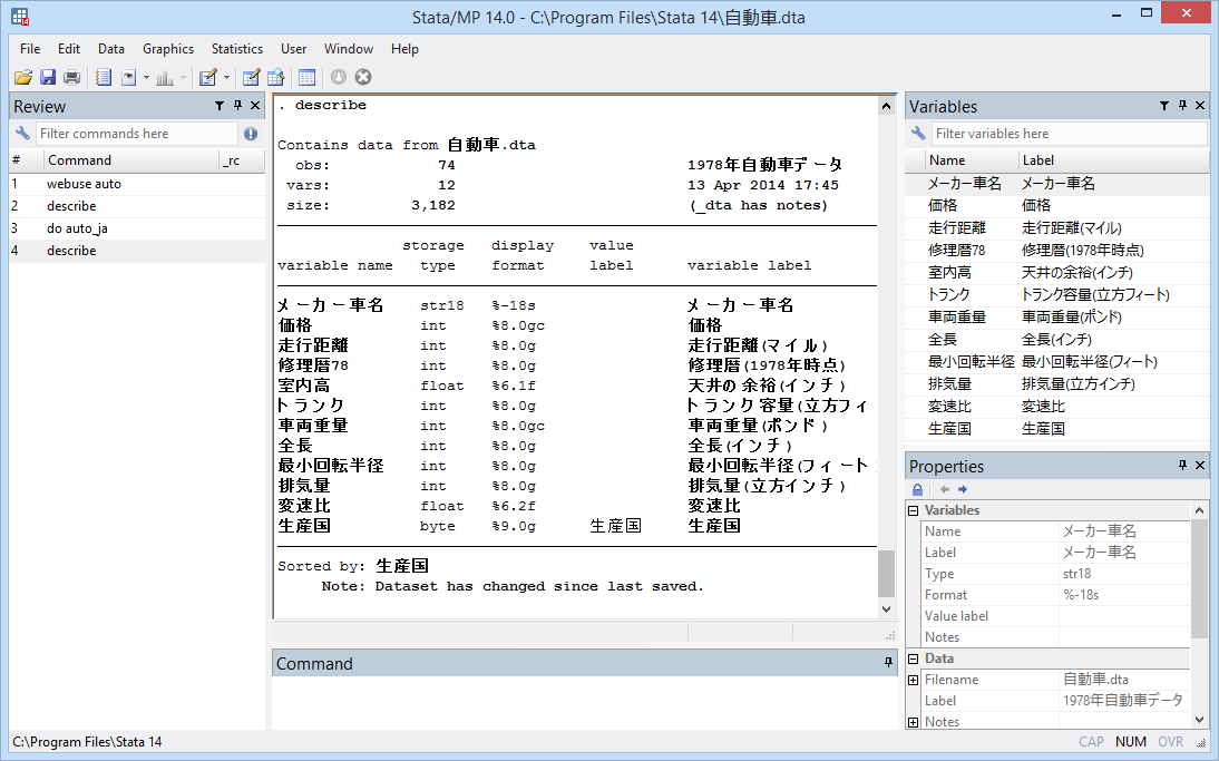
‒ Bill
wgould@stata.com

This post was written jointly with Nikolay Balov, Senior Statistician and Software Developer, StataCorp.

A question on Statalist motivated us to write this blog entry.

A user asked if the churdle command (http://www.stata.com/stata14/hurdle-models/) for fitting hurdle models, new in Stata 14, can be combined with the bayesmh command (http://www.stata.com/stata14/bayesian-analysis/) for fitting Bayesian models, also new in Stata 14:

http://www.statalist.org/forums/forum/general-stata-discussion/general/1290426-comibining-bayesmh-and-churdle

Our initial reaction to this question was ‘No’ or, more precisely, ‘Not easily’ — hurdle models are not among the likelihood models supported by bayesmh. One can write a program to compute the log likelihood of the double hurdle model and use this program with bayesmh (in the spirit of http://www.stata.com/stata14/bayesian-evaluators/), but this may seem like a daunting task if you are not familiar with Stata programming.

And then we realized, why not simply call churdle from the evaluator to compute the log likelihood? All we need is for churdle to evaluate the log likelihood at specific values of model parameters without performing iterations. This can be achieved by specifying churdle‘s options from() and iterate(0).

Let’s look at an example. We consider a simple hurdle model using a subset of the fitness dataset from [R] churdle:

. webuse fitness
. set seed 17653
. sample 10
. churdle linear hours age, select(commute) ll(0)

Iteration 0:   log likelihood = -2783.3352
Iteration 1:   log likelihood =  -2759.029
Iteration 2:   log likelihood = -2758.9992
Iteration 3:   log likelihood = -2758.9992

Cragg hurdle regression                         Number of obs     =      1,983
                                                LR chi2(1)        =       3.42
                                                Prob > chi2       =     0.0645
Log likelihood = -2758.9992                     Pseudo R2         =     0.0006

------------------------------------------------------------------------------
       hours |      Coef.   Std. Err.      z    P>|z|     [95% Conf. Interval]
-------------+----------------------------------------------------------------
hours        |
         age |   .0051263   .0028423     1.80   0.071    -.0004446    .0106971
       _cons |   1.170932   .1238682     9.45   0.000     .9281548    1.413709
-------------+----------------------------------------------------------------
selection_ll |
     commute |  -.0655171   .1561046    -0.42   0.675    -.3714765    .2404423
       _cons |   .1421166   .0882658     1.61   0.107    -.0308813    .3151144
-------------+----------------------------------------------------------------
lnsigma      |
       _cons |   .1280215     .03453     3.71   0.000      .060344     .195699
-------------+----------------------------------------------------------------
      /sigma |   1.136577    .039246                      1.062202    1.216161
------------------------------------------------------------------------------

Let’s assume for a moment that we already have an evaluator, mychurdle1, that returns the corresponding log-likelihood value. We can fit a Bayesian hurdle model using bayesmh as follows:

. gen byte hours0 = (hours==0) //dependent variable for the selection equation
. set seed 123
. bayesmh (hours age) (hours0 commute),
        llevaluator(mychurdle1, parameters({lnsig}))
        prior({hours:} {hours0:} {lnsig}, flat)
        saving(sim, replace) dots

(output omitted)

We use a two-equation specification to fit this model. The main regression is specified first, and the selection regression is specified next. The additional parameter, log of the standard deviation associated with the main regression, is specified in llevaluator()‘s suboption parameters(). All parameters are assigned flat priors to obtain results similar to churdle. MCMC results are saved in sim.dta.

Here is the actual output from bayesmh:

. bayesmh (hours age) (hours0 commute), llevaluator(mychurdle1, parameters({lns
> ig})) prior({hours:} {hours0:} {lnsig}, flat) saving(sim, replace) dots

Burn-in 2500 aaaaaaaaa1000aaaaaa...2000..... done
Simulation 10000 .........1000.........2000.........3000.........4000.........5
> 000.........6000.........7000.........8000.........9000.........10000 done

Model summary
------------------------------------------------------------------------------
Likelihood:
  hours hours0 ~ mychurdle1(xb_hours,xb_hours0,{lnsig})

Priors:
       {hours:age _cons} ~ 1 (flat)                                        (1)
  {hours0:commute _cons} ~ 1 (flat)                                        (2)
                 {lnsig} ~ 1 (flat)
------------------------------------------------------------------------------
(1) Parameters are elements of the linear form xb_hours.
(2) Parameters are elements of the linear form xb_hours0.

Bayesian regression                              MCMC iterations  =     12,500
Random-walk Metropolis-Hastings sampling         Burn-in          =      2,500
                                                 MCMC sample size =     10,000
                                                 Number of obs    =      1,983
                                                 Acceptance rate  =      .2889
                                                 Efficiency:  min =     .05538
                                                              avg =     .06266
Log marginal likelihood = -2772.3953                          max =     .06945

------------------------------------------------------------------------------
             |                                                Equal-tailed
             |      Mean   Std. Dev.     MCSE     Median  [95% Cred. Interval]
-------------+----------------------------------------------------------------
hours        |
         age |  .0050916   .0027972   .000106   .0049923  -.0000372   .0107231
       _cons |  1.167265    .124755   .004889   1.175293   .9125105   1.392021
-------------+----------------------------------------------------------------
hours0       |
     commute | -.0621282   .1549908   .006585  -.0613511  -.3623891   .2379805
       _cons |  .1425693   .0863626   .003313   .1430396  -.0254507   .3097677
-------------+----------------------------------------------------------------
       lnsig |  .1321532   .0346446   .001472   .1326704   .0663646   .2015249
------------------------------------------------------------------------------

file sim.dta saved

The results are similar to those produced by churdle, as one would expect with noninformative priors.

If desired, we can use bayesstats summary to obtain the estimate of the standard deviation:

. bayesstats summary (sigma: exp({lnsig}))

Posterior summary statistics                      MCMC sample size =    10,000

       sigma : exp({lnsig})

------------------------------------------------------------------------------
             |                                                Equal-tailed
             |      Mean   Std. Dev.     MCSE     Median  [95% Cred. Interval]
-------------+----------------------------------------------------------------
       sigma |  1.141969   .0396264   .001685   1.141874   1.068616   1.223267
------------------------------------------------------------------------------

 
Let’s now talk in more detail about a log-likelihood evaluator. We will consider two evaluators: one using churdle and one directly implementing the log likelihood of the considered hurdle model.

Log-likelihood evaluator using churdle

Here we demonstrate how to write a log-likelihood evaluator that calls an existing Stata estimation command, churdle in our example, to compute the log likelihood.

program mychurdle1
        version 14.0
        args llf
        tempname b
        mat `b' = ($MH_b, $MH_p)
        capture churdle linear $MH_y1 $MH_y1x1 if $MH_touse, ///
                    select($MH_y2x1) ll(0) from(`b') iterate(0)
        if _rc {
                if (_rc==1) { // handle break key
                        exit _rc
                }
                scalar `llf' = .
        }
        else {
                scalar `llf' = e(ll)
        }
end

The mychurdle1 program returns the log-likelihood value computed by churdle at the current values of model parameters. This program accepts one argument — a temporary scalar to contain the log-likelihood value llf. We stored current values of model parameters (regression coefficients from two equations stored in vector MH_b and the extra parameter, log standard-deviation, stored in vector MH_p) in a temporary matrix b. We specified churdle‘s options from() and iterate(0) to evaluate the log likelihood at the current parameter values. Finally, we stored the resulting log-likelihood value in llf (or missing value if the command failed to evaluate the log likelihood).

Log-likelihood evaluator directly computing log likelihood

Here we demonstrate how to write a log-likelihood evaluator that computes the likelihood of the fitted hurdle model directly rather than calling churdle.

program mychurdle2
        version 14.0
        args lnf xb xg lnsig
        tempname sig
        scalar `sig' = exp(`lnsig')
        tempvar lnfj
        qui gen double `lnfj' = normal(`xg')  if $MH_touse
        qui replace `lnfj'    = log(1 - `lnfj') if $MH_y1 <= 0 & $MH_touse
        qui replace `lnfj'    = log(`lnfj') - log(normal(`xb'/`sig'))   ///
                              + log(normalden($MH_y1,`xb',`sig'))       ///
                                if $MH_y1 > 0 & $MH_touse
        summarize `lnfj' if $MH_touse, meanonly
        if r(N) < $MH_n {
            scalar `lnf' = .
            exit
        }
        scalar `lnf' = r(sum)
end

The mychurdle2 program accepts four arguments: a temporary scalar to contain the log-likelihood value llf, temporary variables xb and xg containing linear predictors from the corresponding main and selection equations evaluated at the current values of model parameters, and temporary scalar lnsig containing the current value of the log standard-deviation parameter. We compute and store the observation-level log likelihood in a temporary variable lnfj. Global MH_y1 contains the name of the dependent variable from the first (main) equation, and global MH_touse marks the estimation sample. If all observation-specific log likelihood contributions are nonmissing, we store the overall log-likelihood value in lnf or we otherwise store missing.

We fit our model using the same syntax as earlier, except we use mychurdle2 as the program evaluator.

. set seed 123
. bayesmh (hours age) (hours0 commute), llevaluator(mychurdle2, parameters({lns
> ig})) prior({hours:} {hours0:} {lnsig}, flat) saving(sim, replace) dots

Burn-in 2500 aaaaaaaaa1000aaaaaa...2000..... done
Simulation 10000 .........1000.........2000.........3000.........4000.........5
> 000.........6000.........7000.........8000.........9000.........10000 done

Model summary
------------------------------------------------------------------------------
Likelihood:
  hours hours0 ~ mychurdle2(xb_hours,xb_hours0,{lnsig})

Priors:
       {hours:age _cons} ~ 1 (flat)                                        (1)
  {hours0:commute _cons} ~ 1 (flat)                                        (2)
                 {lnsig} ~ 1 (flat)
------------------------------------------------------------------------------
(1) Parameters are elements of the linear form xb_hours.
(2) Parameters are elements of the linear form xb_hours0.

Bayesian regression                              MCMC iterations  =     12,500
Random-walk Metropolis-Hastings sampling         Burn-in          =      2,500
                                                 MCMC sample size =     10,000
                                                 Number of obs    =      1,983
                                                 Acceptance rate  =      .2889
                                                 Efficiency:  min =     .05538
                                                              avg =     .06266
Log marginal likelihood = -2772.3953                          max =     .06945

------------------------------------------------------------------------------
             |                                                Equal-tailed
             |      Mean   Std. Dev.     MCSE     Median  [95% Cred. Interval]
-------------+----------------------------------------------------------------
hours        |
         age |  .0050916   .0027972   .000106   .0049923  -.0000372   .0107231
       _cons |  1.167265    .124755   .004889   1.175293   .9125105   1.392021
-------------+----------------------------------------------------------------
hours0       |
     commute | -.0621282   .1549908   .006585  -.0613511  -.3623891   .2379805
       _cons |  .1425693   .0863626   .003313   .1430396  -.0254507   .3097677
-------------+----------------------------------------------------------------
       lnsig |  .1321532   .0346446   .001472   .1326704   .0663646   .2015249
------------------------------------------------------------------------------

file sim.dta not found; file saved

We obtain the same results as those obtained using approach 1, and we obtain them much faster.

Final remarks

Approach 1 is very straightforward. It can be applied to any Stata command that returns the log likelihood and allows you to specify parameter values at which this log likelihood must be evaluated. Without too much programming effort, you can use almost any existing Stata maximum likelihood estimation command with bayesmh. A disadvantage of approach 1 is slower execution compared with programming the likelihood directly, as in approach 2. For example, the command using the mychurdle1 evaluator from approach 1 took about 25 minutes to run, whereas the command using the mychurdle2 evaluator from approach 2 took only 20 seconds.

This post was written jointly with David Drukker, Director of Econometrics, StataCorp.

The topic for today is the treatment-effects features in Stata.

Treatment-effects estimators estimate the causal effect of a treatment on an outcome based on observational data.

In today’s posting, we will discuss four treatment-effects estimators:

1. RA: Regression adjustment
2. IPW: Inverse probability weighting
3. IPWRA: Inverse probability weighting with regression adjustment
4. AIPW: Augmented inverse probability weighting

We’ll save the matching estimators for part 2.

We should note that nothing about treatment-effects estimators magically extracts causal relationships. As with any regression analysis of observational data, the causal interpretation must be based on a reasonable underlying scientific rationale.

Introduction

We are going to discuss treatments and outcomes.

A treatment could be a new drug and the outcome blood pressure or cholesterol levels. A treatment could be a surgical procedure and the outcome patient mobility. A treatment could be a job training program and the outcome employment or wages. A treatment could even be an ad campaign designed to increase the sales of a product.

Consider whether a mother’s smoking affects the weight of her baby at birth. Questions like this one can only be answered using observational data. Experiments would be unethical.

The problem with observational data is that the subjects choose whether to get the treatment. For example, a mother decides to smoke or not to smoke. The subjects are said to have self-selected into the treated and untreated groups.

In an ideal world, we would design an experiment to test cause-and-effect and treatment-and-outcome relationships. We would randomly assign subjects to the treated or untreated groups. Randomly assigning the treatment guarantees that the treatment is independent of the outcome, which greatly simplifies the analysis.

Causal inference requires the estimation of the unconditional means of the outcomes for each treatment level. We only observe the outcome of each subject conditional on the received treatment regardless of whether the data are observational or experimental. For experimental data, random assignment of the treatment guarantees that the treatment is independent of the outcome; so averages of the outcomes conditional on observed treatment estimate the unconditional means of interest. For observational data, we model the treatment assignment process. If our model is correct, the treatment assignment process is considered as good as random conditional on the covariates in our model.

Let’s consider an example. Figure 1 is a scatterplot of observational data similar to those used by Cattaneo (2010). The treatment variable is the mother’s smoking status during pregnancy, and the outcome is the birthweight of her baby.

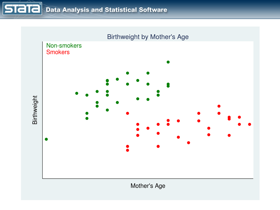
The red points represent the mothers who smoked during pregnancy, while the green points represent the mothers who did not. The mothers themselves chose whether to smoke, and that complicates the analysis.

We cannot estimate the effect of smoking on birthweight by comparing the mean birthweights of babies of mothers who did and did not smoke. Why not? Look again at our graph. Older mothers tend to have heavier babies regardless of whether they smoked while pregnant. In these data, older mothers were also more likely to be smokers. Thus, mother’s age is related to both treatment status and outcome. So how should we proceed?

RA: The regression adjustment estimator

RA estimators model the outcome to account for the nonrandom treatment assignment.

We might ask, “How would the outcomes have changed had the mothers who smoked chosen not to smoke?” or “How would the outcomes have changed had the mothers who didn’t smoke chosen to smoke?”. If we knew the answers to these counterfactual questions, analysis would be easy: we would just subtract the observed outcomes from the counterfactual outcomes.

The counterfactual outcomes are called unobserved potential outcomes in the treatment-effects literature. Sometimes the word unobserved is dropped.

We can construct measurements of these unobserved potential outcomes, and our data might look like this:

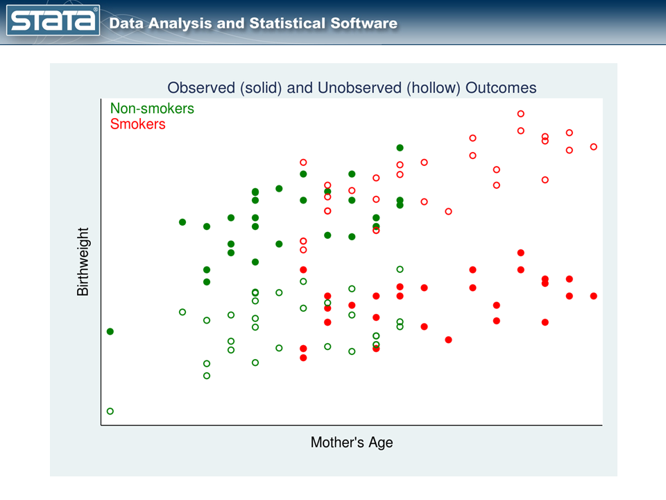
In figure 2, the observed data are shown using solid points and the unobserved potential outcomes are shown using hollow points. The hollow red points represent the potential outcomes for the smokers had they not smoked. The hollow green points represent the potential outcomes for the nonsmokers had they smoked.

We can estimate the unobserved potential outcomes then by fitting separate linear regression models with the observed data (solid points) to the two treatment groups.

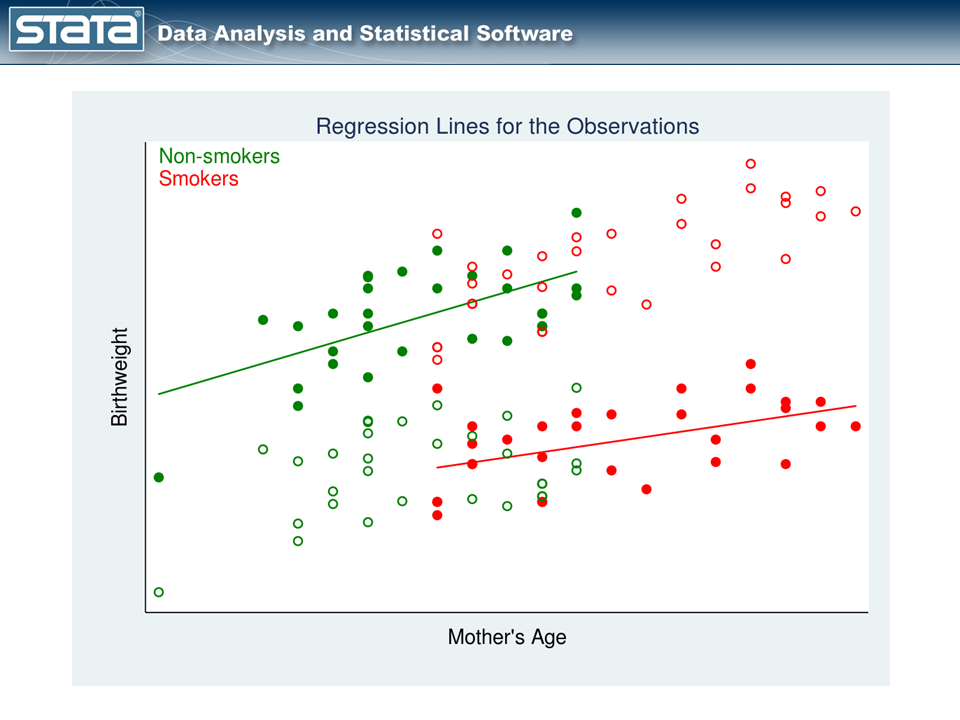
In figure 3, we have one regression line for nonsmokers (the green line) and a separate regression line for smokers (the red line).

Let’s understand what the two lines mean:

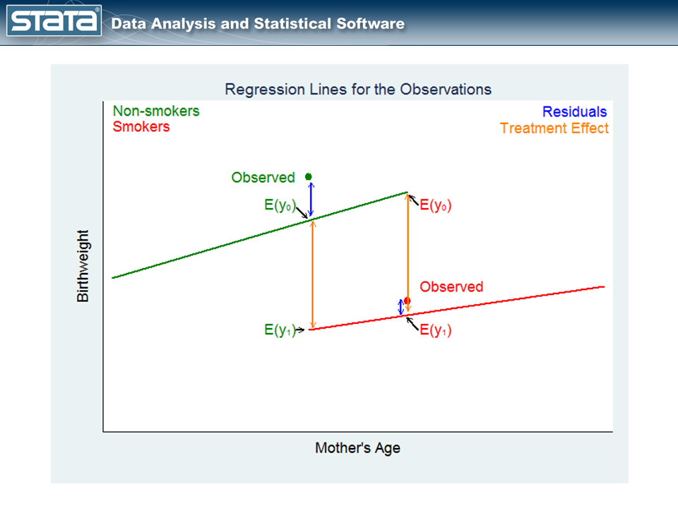
The green point on the left in figure 4, labeled Observed, is an observation for a mother who did not smoke. The point labeled E(y0) on the green regression line is the expected birthweight of the baby given the mother’s age and that she didn’t smoke. The point labeled E(y1) on the red regression line is the expected birthweight of the baby for the same mother had she smoked.

The difference between these expectations estimates the covariate-specific treatment effect for those who did not get the treatment.

Now, let’s look at the other counterfactual question.

The red point on the right in figure 4, labeled Observed in red, is an observation for a mother who smoked during pregnancy. The points on the green and red regression lines again represent the expected birthweights — the potential outcomes — of the mother’s baby under the two treatment conditions.

The difference between these expectations estimates the covariate-specific treatment effect for those who got the treatment.

Note that we estimate an average treatment effect (ATE), conditional on covariate values, for each subject. Furthermore, we estimate this effect for each subject, regardless of which treatment was actually received. Averages of these effects over all the subjects in the data estimate the ATE.

We could also use figure 4 to motivate a prediction of the outcome that each subject would obtain for each treatment level, regardless of the treatment recieved. The story is analogous to the one above. Averages of these predictions over all the subjects in the data estimate the potential-outcome means (POMs) for each treatment level.

It is reassuring that differences in the estimated POMs is the same estimate of the ATE discussed above.

The ATE on the treated (ATET) is like the ATE, but it uses only the subjects who were observed in the treatment group. This approach to calculating treatment effects is called regression adjustment (RA).

Let’s open a dataset and try this using Stata.

. webuse cattaneo2.dta, clear
(Excerpt from Cattaneo (2010) Journal of Econometrics 155: 138-154)

To estimate the POMs in the two treatment groups, we type

. teffects ra (bweight mage) (mbsmoke), pomeans

We specify the outcome model in the first set of parentheses with the outcome variable followed by its covariates. In this example, the outcome variable is bweight and the only covariate is mage.

We specify the treatment model — simply the treatment variable — in the second set of parentheses. In this example, we specify only the treatment variable mbsmoke. We’ll talk about covariates in the next section.

The result of typing the command is

. teffects ra (bweight mage) (mbsmoke), pomeans

Iteration 0:   EE criterion =  7.878e-24
Iteration 1:   EE criterion =  8.468e-26

Treatment-effects estimation                    Number of obs      =      4642
Estimator      : regression adjustment
Outcome model  : linear
Treatment model: none
------------------------------------------------------------------------------
             |               Robust
     bweight |      Coef.   Std. Err.      z    P>|z|     [95% Conf. Interval]
-------------+----------------------------------------------------------------
POmeans      |
     mbsmoke |
  nonsmoker  |   3409.435   9.294101   366.84   0.000     3391.219    3427.651
     smoker  |   3132.374   20.61936   151.91   0.000     3091.961    3172.787
------------------------------------------------------------------------------

The output reports that the average birthweight would be 3,132 grams if all mothers smoked and 3,409 grams if no mother smoked.

We can estimate the ATE of smoking on birthweight by subtracting the POMs: 3132.374 – 3409.435 = -277.061. Or we can reissue our teffects ra command with the ate option and get standard errors and confidence intervals:

. teffects ra (bweight mage) (mbsmoke), ate

Iteration 0:   EE criterion =  7.878e-24
Iteration 1:   EE criterion =  5.185e-26

Treatment-effects estimation                    Number of obs      =      4642
Estimator      : regression adjustment
Outcome model  : linear
Treatment model: none
-------------------------------------------------------------------------------
              |               Robust   
      bweight |      Coef.   Std. Err.      z    P>|z|     [95% Conf. Interval]
--------------+----------------------------------------------------------------
ATE           |        
      mbsmoke |
(smoker vs    |        
  nonsmoker)  |  -277.0611   22.62844   -12.24   0.000    -321.4121   -232.7102
--------------+----------------------------------------------------------------
POmean        |        
      mbsmoke |
   nonsmoker  |   3409.435   9.294101   366.84   0.000     3391.219    3427.651
-------------------------------------------------------------------------------

The output reports the same ATE we calculated by hand: -277.061. The ATE is the average of the differences between the birthweights when each mother smokes and the birthweights when no mother smokes.

We can also estimate the ATET by using the teffects ra command with option atet, but we will not do so here.

IPW: The inverse probability weighting estimator

RA estimators model the outcome to account for the nonrandom treatment assignment. Some researchers prefer to model the treatment assignment process and not specify a model for the outcome.

We know that smokers tend to be older than nonsmokers in our data. We also hypothesize that mother’s age directly affects birthweight. We observed this in figure 1, which we show again below.

This figure shows that treatment assignment depends on mother’s age. We would like to have a method of adjusting for this dependence. In particular, we wish we had more upper-age green points and lower-age red points. If we did, the mean birthweight for each group would change. We don’t know how that would affect the difference in means, but we do know it would be a better estimate of the difference.

To achieve a similar result, we are going to weight smokers in the lower-age range and nonsmokers in the upper-age range more heavily, and weight smokers in the upper-age range and nonsmokers in the lower-age range less heavily.

We will fit a probit or logit model of the form

Pr(woman smokes) = F(a + b*age)

teffects uses logit by default, but we will specify the probit option for illustration.

Once we have fit that model, we can obtain the prediction Pr(woman smokes) for each observation in the data; we’ll call this p_i. Then, in making our POMs calculations — which is just a mean calculation — we will use those probabilities to weight the observations. We will weight observations on smokers by 1/p_i so that weights will be large when the probability of being a smoker is small. We will weight observations on nonsmokers by 1/(1-p_i) so that weights will be large when the probability of being a nonsmoker is small.

That results in the following graph replacing figure 1:

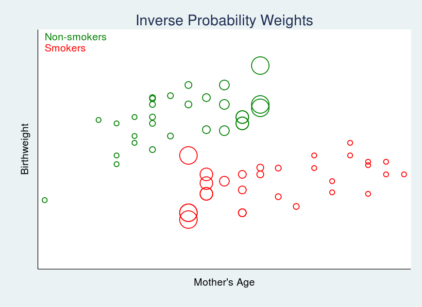
In figure 5, larger circles indicate larger weights.

To estimate the POMs with this IPW estimator, we can type

. teffects ipw (bweight) (mbsmoke mage, probit), pomeans

The first set of parentheses specifies the outcome model, which is simply the outcome variable in this case; there are no covariates. The second set of parentheses specifies the treatment model, which includes the outcome variable (mbsmoke) followed by covariates (in this case, just mage) and the kind of model (probit).

The result is

. teffects ipw (bweight) (mbsmoke mage, probit), pomeans

Iteration 0:   EE criterion =  3.615e-15
Iteration 1:   EE criterion =  4.381e-25

Treatment-effects estimation                    Number of obs      =      4642
Estimator      : inverse-probability weights
Outcome model  : weighted mean
Treatment model: probit
------------------------------------------------------------------------------
             |               Robust
     bweight |      Coef.   Std. Err.      z    P>|z|     [95% Conf. Interval]
-------------+----------------------------------------------------------------
POmeans      |
     mbsmoke |
  nonsmoker  |   3408.979   9.307838   366.25   0.000     3390.736    3427.222
     smoker  |   3133.479   20.66762   151.61   0.000     3092.971    3173.986
------------------------------------------------------------------------------

Our output reports that the average birthweight would be 3,133 grams if all the mothers smoked and 3,409 grams if none of the mothers smoked.

This time, the ATE is -275.5, and if we typed

. teffects ipw (bweight) (mbsmoke mage, probit), ate
(Output omitted)

we would learn that the standard error is 22.68 and the 95% confidence interval is [-319.9,231.0].

Just as with teffects ra, if we wanted ATET, we could specify the teffects ipw command with the atet option.

IPWRA: The IPW with regression adjustment estimator

RA estimators model the outcome to account for the nonrandom treatment assignment. IPW estimators model the treatment to account for the nonrandom treatment assignment. IPWRA estimators model both the outcome and the treatment to account for the nonrandom treatment assignment.

IPWRA uses IPW weights to estimate corrected regression coefficients that are subsequently used to perform regression adjustment.

The covariates in the outcome model and the treatment model do not have to be the same, and they often are not because the variables that influence a subject’s selection of treatment group are often different from the variables associated with the outcome. The IPWRA estimator has the double-robust property, which means that the estimates of the effects will be consistent if either the treatment model or the outcome model — but not both — are misspecified.

Let’s consider a situation with more complex outcome and treatment models but still using our low-birthweight data.

The outcome model will include

1. mage: the mother’s age
2. prenatal1: an indicator for prenatal visit during the first trimester
3. mmarried: an indicator for marital status of the mother
4. fbaby: an indicator for being first born

The treatment model will include

1. all the covariates of the outcome model
2. mage^2
3. medu: years of maternal education

We will also specify the aequations option to report the coefficients of the outcome and treatment models.

. teffects ipwra (bweight mage prenatal1 mmarried fbaby)                ///
                 (mbsmoke mmarried c.mage##c.mage fbaby medu, probit)   ///
                 , pomeans aequations

Iteration 0:   EE criterion =  1.001e-20
Iteration 1:   EE criterion =  1.134e-25

Treatment-effects estimation                    Number of obs      =      4642
Estimator      : IPW regression adjustment
Outcome model  : linear
Treatment model: probit
-------------------------------------------------------------------------------
              |               Robust
      bweight |      Coef.   Std. Err.      z    P>|z|     [95% Conf. Interval]
--------------+----------------------------------------------------------------
POmeans       |
      mbsmoke |
   nonsmoker  |   3403.336    9.57126   355.58   0.000     3384.576    3422.095
      smoker  |   3173.369   24.86997   127.60   0.000     3124.624    3222.113
--------------+----------------------------------------------------------------
OME0          |
         mage |   2.893051   2.134788     1.36   0.175    -1.291056    7.077158
    prenatal1 |   67.98549   28.78428     2.36   0.018     11.56933    124.4017
     mmarried |   155.5893   26.46903     5.88   0.000      103.711    207.4677
        fbaby |   -71.9215   20.39317    -3.53   0.000    -111.8914   -31.95162
        _cons |   3194.808   55.04911    58.04   0.000     3086.913    3302.702
--------------+----------------------------------------------------------------
OME1          |
         mage |  -5.068833   5.954425    -0.85   0.395    -16.73929    6.601626
    prenatal1 |   34.76923   43.18534     0.81   0.421    -49.87248    119.4109
     mmarried |   124.0941   40.29775     3.08   0.002     45.11193    203.0762
        fbaby |   39.89692   56.82072     0.70   0.483    -71.46966    151.2635
        _cons |   3175.551   153.8312    20.64   0.000     2874.047    3477.054
--------------+----------------------------------------------------------------
TME1          |
     mmarried |  -.6484821   .0554173   -11.70   0.000     -.757098   -.5398663
         mage |   .1744327   .0363718     4.80   0.000     .1031452    .2457202
              |
c.mage#c.mage |  -.0032559   .0006678    -4.88   0.000    -.0045647   -.0019471
              |
        fbaby |  -.2175962   .0495604    -4.39   0.000    -.3147328   -.1204595
         medu |  -.0863631   .0100148    -8.62   0.000    -.1059917   -.0667345
        _cons |  -1.558255   .4639691    -3.36   0.001    -2.467618   -.6488926
-------------------------------------------------------------------------------

The POmeans section of the output displays the POMs for the two treatment groups. The ATE is now calculated to be 3173.369 – 3403.336 = -229.967.

The OME0 and OME1 sections display the RA coefficients for the untreated and treated groups, respectively.

The TME1 section of the output displays the coefficients for the probit treatment model.

Just as in the two previous cases, if we wanted the ATE with standard errors, etc., we would specify the ate option. If we wanted ATET, we would specify the atet option.

AIPW: The augmented IPW estimator

IPWRA estimators model both the outcome and the treatment to account for the nonrandom treatment assignment. So do AIPW estimators.

The AIPW estimator adds a bias-correction term to the IPW estimator. If the treatment model is correctly specified, the bias-correction term is 0 and the model is reduced to the IPW estimator. If the treatment model is misspecified but the outcome model is correctly specified, the bias-correction term corrects the estimator. Thus, the bias-correction term gives the AIPW estimator the same double-robust property as the IPWRA estimator.

The syntax and output for the AIPW estimator is almost identical to that for the IPWRA estimator.

. teffects aipw (bweight mage prenatal1 mmarried fbaby)                 ///
                (mbsmoke mmarried c.mage##c.mage fbaby medu, probit)    ///
                , pomeans aequations

Iteration 0:   EE criterion =  4.632e-21
Iteration 1:   EE criterion =  5.810e-26

Treatment-effects estimation                    Number of obs      =      4642
Estimator      : augmented IPW
Outcome model  : linear by ML
Treatment model: probit
-------------------------------------------------------------------------------
              |               Robust
      bweight |      Coef.   Std. Err.      z    P>|z|     [95% Conf. Interval]
--------------+----------------------------------------------------------------
POmeans       |
      mbsmoke |
   nonsmoker  |   3403.355   9.568472   355.68   0.000     3384.601    3422.109
      smoker  |   3172.366   24.42456   129.88   0.000     3124.495    3220.237
--------------+----------------------------------------------------------------
OME0          |
         mage |   2.546828   2.084324     1.22   0.222    -1.538373    6.632028
    prenatal1 |   64.40859   27.52699     2.34   0.019     10.45669    118.3605
     mmarried |   160.9513    26.6162     6.05   0.000     108.7845    213.1181
        fbaby |   -71.3286   19.64701    -3.63   0.000     -109.836   -32.82117
        _cons |   3202.746   54.01082    59.30   0.000     3096.886    3308.605
--------------+----------------------------------------------------------------
OME1          |
         mage |  -7.370881    4.21817    -1.75   0.081    -15.63834    .8965804
    prenatal1 |   25.11133   40.37541     0.62   0.534    -54.02302    104.2457
     mmarried |   133.6617   40.86443     3.27   0.001      53.5689    213.7545
        fbaby |   41.43991   39.70712     1.04   0.297    -36.38461    119.2644
        _cons |   3227.169   104.4059    30.91   0.000     3022.537    3431.801
--------------+----------------------------------------------------------------
TME1          |
     mmarried |  -.6484821   .0554173   -11.70   0.000     -.757098   -.5398663
         mage |   .1744327   .0363718     4.80   0.000     .1031452    .2457202
              |
c.mage#c.mage |  -.0032559   .0006678    -4.88   0.000    -.0045647   -.0019471
              |
        fbaby |  -.2175962   .0495604    -4.39   0.000    -.3147328   -.1204595
         medu |  -.0863631   .0100148    -8.62   0.000    -.1059917   -.0667345
        _cons |  -1.558255   .4639691    -3.36   0.001    -2.467618   -.6488926
-------------------------------------------------------------------------------

The ATE is 3172.366 – 3403.355 = -230.989.

Final thoughts

The example above used a continuous outcome: birthweight. teffects can also be used with binary, count, and nonnegative continuous outcomes.

The estimators also allow multiple treatment categories.

An entire manual is devoted to the treatment-effects features in Stata 13, and it includes a basic introduction, advanced discussion, and worked examples. If you would like to learn more, you can download the [TE] Treatment-effects Reference Manual from the Stata website.

More to come

Next time, in part 2, we will cover the matching estimators.

Reference

Cattaneo, M. D. 2010. Efficient semiparametric estimation of multi-valued treatment effects under ignorability. Journal of Econometrics 155: 138–154.

New to Stata 14 is a suite of commands to fit item response theory (IRT) models. IRT models are used to analyze the relationship between the latent trait of interest and the items intended to measure the trait. Stata’s irt commands provide easy access to some of the commonly used IRT models for binary and polytomous responses, and irtgraph commands can be used to plot item characteristic functions and information functions.

To learn more about Stata’s IRT features, I refer you to the [IRT] manual; here I want to go beyond the manual and show you a couple of examples of what you can do with a little bit of Stata code.

Example 1

To get started, I want to show you how simple IRT analysis is in Stata.

When I use the nine binary items q1–q9, all I need to type to fit a 1PL model is

irt 1pl q*

Equivalently, I can use a dash notation or explicitly spell out the variable names:

irt 1pl q1-q9
irt 1pl q1 q2 q3 q4 q5 q6 q7 q8 q9

I can also use parenthetical notation:

irt (1pl q1-q9)

Parenthetical notation is not very useful for a simple IRT model, but comes in handy when you want to fit a single IRT model to combinations of binary, ordinal, and nominal items:

irt (1pl q1-q5) (1pl q6-q9) (pcm x1-x10) ...

IRT graphs are equally simple to create in Stata; for example, to plot item characteristic curves (ICCs) for all the items in a model, I type

irtgraph icc

Yes, that’s it!

Example 2

Sometimes, I want to fit the same IRT model on two different groups and see how the estimated parameters differ between the groups. The exercise can be part of investigating differential item functioning (DIF) or parameter invariance.

I split the data into two groups, fit two separate 2PL models, and create two scatterplots to see how close the parameter estimates for discrimination and difficulty are for the two groups. For simplicity, my group variable is 1 for odd-numbered observations and 0 for even-numbered observations.

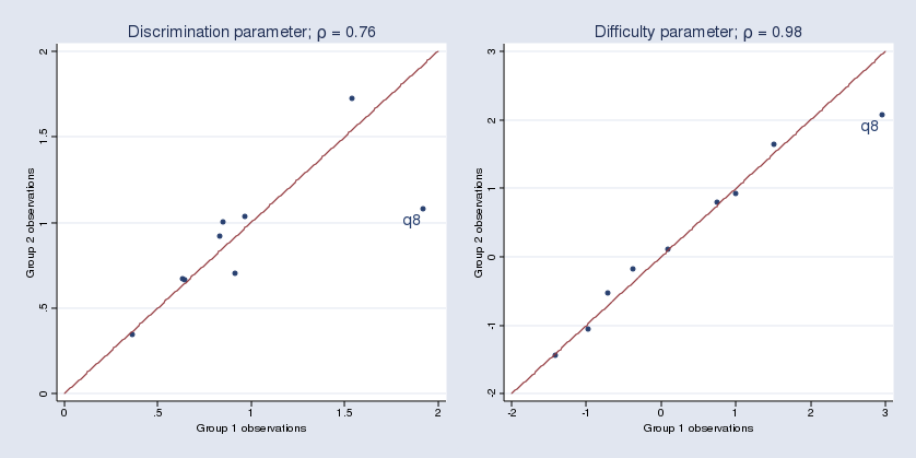
We see that the estimated parameters for item q8 appear to differ between the two groups.

Here is the code used in this example.

webuse masc1, clear

gen odd = mod(_n,2)

irt 2pl q* if odd
mat b_odd = e(b)'

irt 2pl q* if !odd
mat b_even = e(b)'

svmat double b_odd, names(group1)
svmat double b_even, names(group2)
replace group11 = . in 19
replace group21 = . in 19

gen lab1 = ""
replace lab1 = "q8" in 15

gen lab2 = ""
replace lab2 = "q8" in 16

corr group11 group21 if mod(_n,2)
local c1 : display %4.2f `r(rho)'

twoway (scatter group11 group21, mlabel(lab1) mlabsize(large) mlabpos(7)) ///
        (function x, range(0 2)) if mod(_n,2), ///
        name(discr,replace) title("Discrimination parameter; {&rho} = `c1'") ///
        xtitle("Group 1 observations") ytitle("Group 2 observations") ///
        legend(off)

corr group11 group21 if !mod(_n,2)
local c2 : display %4.2f `r(rho)'

twoway (scatter group11 group21, mlabel(lab2) mlabsize(large) mlabpos(7)) ///
        (function x, range(-2 3)) if !mod(_n,2), ///
        name(diff,replace) title("Difficulty parameter; {&rho} = `c2'") ///
        xtitle("Group 1 observations") ytitle("Group 2 observations") ///
        legend(off)

graph combine discr diff, xsize(8)

Example 3

Continuing with the example above, I want to show you how to use a likelihood-ratio test to test for item parameter differences between groups.

Using item q8 as an example, I want to fit one model that constrains item q8 parameters to be the same between the two groups and fit another model that allows these parameters to vary.

The first model is easy. I can fit a 2PL model for the entire dataset, which implicitly constrains the parameters to be equal for both groups. I store the estimates under the name equal.

. webuse masc1, clear
(Data from De Boeck & Wilson (2004))

. generate odd = mod(_n,2)
. quietly irt 2pl q*
. estimates store equal

To estimate the second model, I need the following:

. irt (2pl q1-q7 q9) (2pl q8 if odd) (2pl q8 if !odd)

Unfortunately, this is illegal syntax. I can, however, split the item into two new variables where each variable is restricted to the required subsample:

. generate q8_1 = q8 if odd
(400 missing values generated)

. generate q8_2 = q8 if !odd
(400 missing values generated)

I estimate the second IRT model, this time with items q8_1 and q8_2 taking place of the original q8:

. quietly irt 2pl q1-q7 q8_1 q8_2 q9
. estat report q8_1 q8_2

Two-parameter logistic model                    Number of obs     =        800
Log likelihood = -4116.2064
------------------------------------------------------------------------------
             |      Coef.   Std. Err.      z    P>|z|     [95% Conf. Interval]
-------------+----------------------------------------------------------------
q8_1         |
     Discrim |   1.095867   .2647727     4.14   0.000     .5769218    1.614812
        Diff |  -1.886126   .3491548    -5.40   0.000    -2.570457   -1.201795
-------------+----------------------------------------------------------------
q8_2         |
     Discrim |    1.93005   .4731355     4.08   0.000     1.002721    2.857378
        Diff |  -1.544908   .2011934    -7.68   0.000     -1.93924   -1.150577
------------------------------------------------------------------------------

Now, I can perform the likelihood-ratio test:

. lrtest equal ., force

Likelihood-ratio test                                 LR chi2(2)  =      4.53
(Assumption: equal nested in .)                       Prob > chi2 =    0.1040

The test suggests the first model is preferable even though the two ICCs clearly differ:

. irtgraph icc q8_1 q8_2, ylabel(0(.25)1)

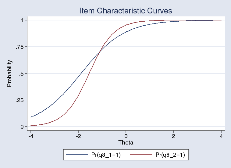
Summary

IRT models are used to analyze the relationship between the latent trait of interest and the items intended to measure the trait. Stata’s irt commands provide easy access to some of the commonly used IRT models, and irtgraph commands implement the most commonly used IRT plots. With just a few extra steps, you can easily create customized graphs, such as the ones demonstrated above, which incorporate information from separate IRT models.